Choice of Symplectic Integrator in Hamiltonian Monte Carlo

This is the fourth post in a series exploring implementing gradient based samplers in practice. Background is available on automatic differentiation, a basic implementation of Hamiltonian Monte Carlo, and step size adaptation for MCMC. A well tested, documented library containing all of this code is available here. Pull requests and issues are welcome.

This is a bit of a deep dive into our choice of integrator in Hamiltonian Monte Carlo (HMC). As a spoiler alert, we find that the leapfrog integrator is empirically the fastest, or at least no slower, than other integrators. It is still interesting to consider what choice we have made, and why we have made it.

Much of the material here is from Janne Mannseth, Tore Selland Kleppe, and Hans J. Skaug in On the Application of Higher Order Symplectic Integrators in Hamiltonian Monte Carlo, as implemented by Adrian Seyboldt in PyMC3.

A very brief reminder about HMC

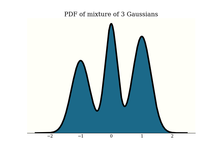
Recall that in HMC, we have a probability density function $\pi$ defined on $\mathbb{R}^n$, and wish to generate samples from it. This is the distribution I will use for examples today: it is a mixture of 3 Gaussians:

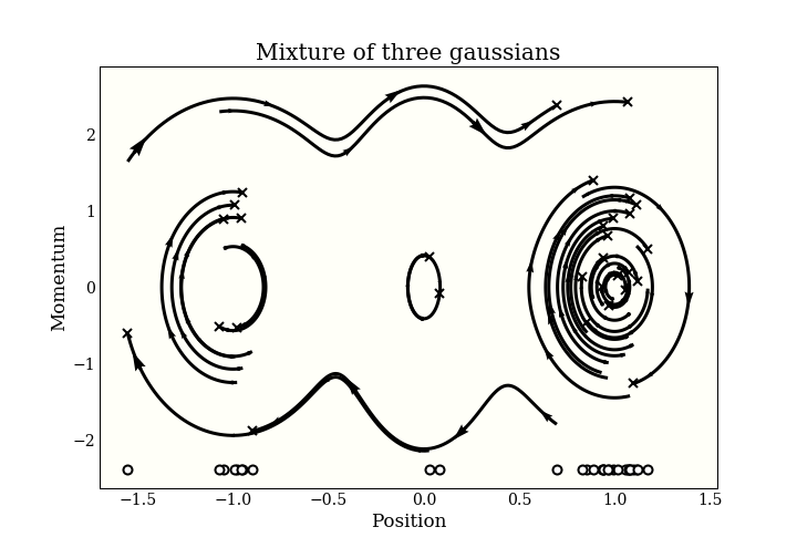
To generate samples with HMC, we add an $n$-dimensional momentum variable, then simulate some physics in $\mathbb{R}^{2n}$. The physics goes on in this “(position, momentum) space”. To get our MCMC samples, we just forget the momentum and keep the position. Here is a picture of some samples in (position, momentum) space:

The end of each trajectory is marked with an x, and the actual samples are marked on the bottom of the plot. You can see the start of the 3 modes forming!

A naive integrator

Let’s first implement the most obvious thing, to convince ourselves that we want to improve it. The Hamiltonian equations simplify to $$ \frac{d \mathbf{q}}{dt} = \mathbf{p} \\
\frac{d \mathbf{p}}{dt} = - \frac{\partial V}{\partial \mathbf{q}} $$ where $V = -\log \pi(\mathbf{q})$.

Then given

• an initial position q and initial momentum p,
• a step size step_size,
• and a path length path_len,

a straightforward approach is

for _ in range(int(path_len / step_size)):
    p -= step_size * dVdq(q)  # update momentum
    q += step_size * p  # update position

How does this look graphically in (position, momentum) space?

The first cell shows the exact path that the integrator is trying to follow: the green triangle is the start, and the red target is where the new proposal should be. The second plot shows each step the integrator makes. It does not do that well! The red “X” shows where it ended up, which is kind of far from the target. The third plot shows each intermediate step: a full momentum update (vertical move), followed by a full position update (horizontal move). Notice that every other move lies on the trajectory of the integrator.

In addition to the accuracy, we should keep in mind the computational cost, since this is going to be an inner loop in running MCMC. This algorithm does 1 gradient evaluation per step.

To do better, we move to a class of integrators with a special volume preserving property.

What is a symplectic integrator?

I did not do a deep dive into symplectic integrators, spending most of my time on numerical experiments, so I am a little nervous about this section. Remember to always consult a mathematician before engaging in any symplectic integration.

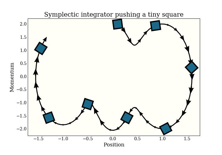
I will give the somewhat-imprecise definition of a symplectic integrator as one that preserves volume. Specifically, if you take a (infinetessimal) square and apply the integrator to it, the square will maintain the same (infinitessimal) volume. This condition is very similar to a technical condition that is sufficient to define an MCMC sampler.

Remember that this chart - and the symplectic property - is in (position, momentum) space.

A first symplectic integrator: the leapfrog integrator

As an example (without proof!) of a symplectic integrator, here is the leapfrog integrator. This is the one actually used in HMC in every practical implementation I have seen (Stan, PyMC3, Pyro, TensorFlow Probability, Ranier). See the benchmarks at the end of the article, and also this thoughtful discussion between the wonderful Adrian Seyboldt and Bob Carpenter on the practical use of higher order integrators, which matches my experience.

The only difference between a leapfrog integrator and the naive integrator above is that we start with a half momentum update, then a full position update, then another half update (whence “leapfrog”):

for _ in np.arange(np.round(path_len / step_size)):
    p -= step_size * dVdq(q) / 2  # half momentum update
    q += step_size * p  # whole position update
    p -= step_size * dVdq(q) / 2  # half momentum update

Note that this costs two gradient evaluations per loop, but a simple change can make it twice as fast by combining the half updates in the loop:

p -= step_size * dVdq(q) / 2  # half momentum update
for _ in np.arange(np.round(path_len / step_size) - 1):
    q += step_size * p  # whole position update
    p -= step_size * dVdq(q)  # whole momentum update
q += step_size * p  # whole position update
p -= step_size * dVdq(q) / 2  # half momentum update

Now the cost is the same 1 gradient per step (plus a single extra gradient evaluation, amortized over all the steps). We can look at the performance in the same way as the naive integrator:

By interleaving the half steps, the leapfrog integrator does better at tracking the true trajectory, with essentially the same cost.

Two-stage leapfrog

A two-stage integrator makes 2 leapfrog steps per update. The distance of each update is calculated to keep the symplectic property (this fact should not be clear, but it is important):

for _ in np.arange(np.round(path_len / step_size)):
    p -= C * step_size * dVdq(q)  # `C` momentum update
    q += step_size * p / 2  # half position update
    p -= (1 - 2 * C) * step_size * dVdq(q)  # 1 - 2C position update
    q += step_size * p / 2  # half position update
    p -= C * step_size * dVdq(q)  # `a` momentum update

There is a constant C there chosen to maximize the acceptance probability, and the value, $\frac{3 - \sqrt{3}}{6}$, is not important.

Note also that we can do the same loop wrapping trick, so this two-stage leapfrog takes 2 gradient evaluations per step. We show in the benchmarks that the added expense almost, but does not quite, pay for itself.

Three-stage leapfrog

As a final experiment, we show a symplectic integrator with three leapfrog steps per update. This time there are two constants that are not important, but kind of wild if you are that kind of person at parties ($\frac{12,127,897}{102,017,882}$ and $\frac{4,271,554}{14,421,423}$). We call them C and D below.

for _ in np.arange(np.round(path_len / step_size)):
    p -= C * step_size * dVdq(q)  # C step
    q += D * step_size * p  # D step
    p -= (0.5 - C) * step_size * dVdq(q)  # (0.5 - C) step
    q += (1 - 2 * D) * step_size * p  # (1 - 2D) step
    p -= (0.5 - C) * step_size * dVdq(q) # (0.5 - C) step
    q += D * step_size * p  # D step
    p -= C * step_size * dVdq(q)  # C step

This will end up costing 3 gradient evaluations per update once we wrap the gradient at the end of the loop.

Just for fun, here is also the three-stage integrator with a step size twice as big as above

Compare this to all the other integrators, which make bad mistakes with such a large step:

Which integrator to use?

Benchmarking MCMC is hard. Three big problems you should have with my method here are:

1. I should test on real data as well as simulated data. But I have not made an API that is good at handling real data yet.
2. I should benchmark effective sample size per second. But I have not implemented parallel sampling yet, and I have things to do with my computer that don’t involve simulations for blog posts.
3. I should test on probability densities with more complicated geometry, like hierarchical models. But I have not yet implemented divergence handling, and this goes… poorly.

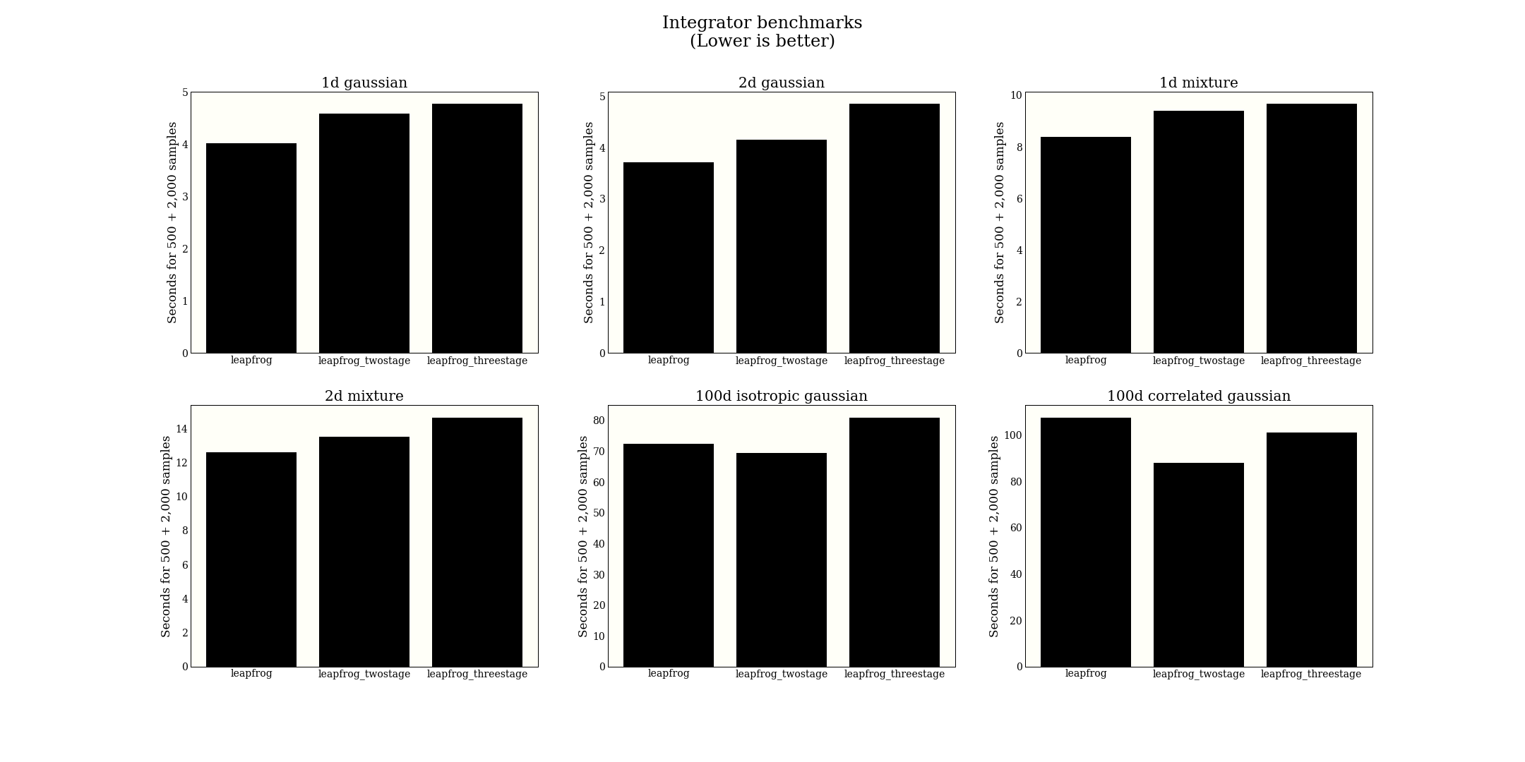
Given what tools I do have, I put together 6 test distributions, and run the following experiment for each distribution:

1. Fix a path length (this is plausibly similar to producing the same effective sample size)
2. Automatically tune step size to get a rate of 0.7
3. Draw 2,000 samples
4. Report the time for both the tuning and the sampling

The figure displays a little small, but right click to open in a new tab to see better.

From this big experiment, I conclude that the regular leapfrog is perhaps better, or at least comparable with higher-order leapfrog methods. In terms of implementation, it is much simpler, so we might as well use it. Note that the paper claims efficiency gains in NUTS, which is optimized a bit differently from HMC, so I am not contradicting that claim.