The notebook that generated this blog post can be found here
This is a short note on how to use an automatic differentiation library, starting from exercises that feel like calculus, and ending with an application to linear regression using very basic gradient descent.
I am using autograd here, though these experiments were originally done using jax, which adds XLA support, so everything can run on the GPU. It is strikingly easy to move from autograd to jax, but the random number generation is just weird enough that the following is run with autograd. I have included the equivalent jax code for everyting, though
Automatic differentiation has found intense application in deep learning, but my interest is in probabilistic programming, and gradient-based Markov chain Monte Carlo in particular. There are a number of probabilistic programming libraries built on top of popular deep learning libraries, reaping the benefits of efficient gradients and computation:
The Stan library implements their own automatic differentiation.
At their simplest, these libraries both work by taking a function $f: \mathbb{R}^n \rightarrow \mathbb{R}$ and return the gradient, $\nabla f: \mathbb{R}^n \rightarrow \mathbb{R}^n$. This can be chained to get second or third derivatives.
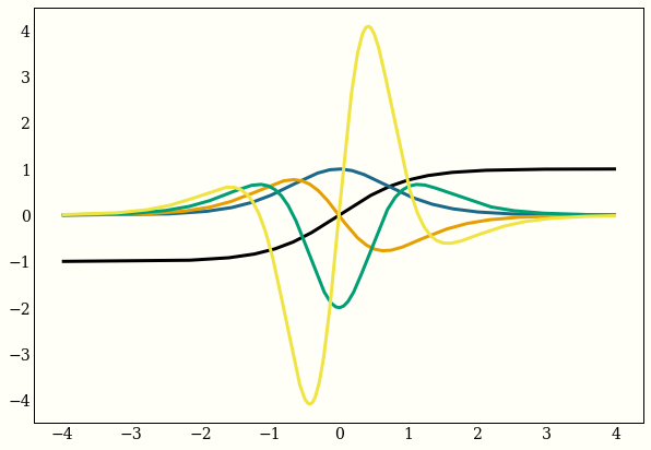
Example 1: Derivatives of a function
Here are the first 4 derivatives of the hyperbolic tangent:
import matplotlib.pyplot as plt
import autograd.numpy as np
from autograd import elementwise_grad

fig, ax = plt.subplots(figsize=(10, 7))

x = np.linspace(-4, 4, 1000)

my_func = np.tanh
ax.plot(x, my_func(x))
for _ in range(4):
    my_func = elementwise_grad(my_func)
    ax.plot(x, my_func(x))
Note: the equivalent code in jax is
import jax.numpy as np
from jax import grad, vmap

fig, ax = plt.subplots(figsize=(10, 7))

x = np.linspace(-4, 4, 1000)

my_func = np.tanh
ax.plot(x, my_func(x))
for _ in range(4):
    my_func = grad(my_func)
    ax.plot(x, vmap(my_func)(x))
The difference being that we have vmap instead of elementwise_grad, so we take all our gradients, and then map the function across a vector.
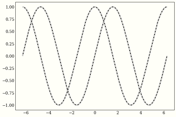
Example 2: Trig functions
My favorite way of defining trigonometric functions like sine and cosine are as solutions to the differential equation $$ y” = -y $$
We can use autograd to confirm that sine and cosine both satisfy this equality.
fig, ax = plt.subplots(figsize=(10, 7))

x = np.linspace(-2 * np.pi, 2 * np.pi, 1000)

for func in (np.sin, np.cos):
    second_derivative = elementwise_grad(elementwise_grad(func))
    ax.plot(x, func(x), 'k-')
    ax.plot(x, -second_derivative(x), 'w--', lw=2)
Again, the equivalent jax code just maps vmap to elementwise_grad:
fig, ax = plt.subplots(figsize=(10, 7))

x = np.linspace(-2 * np.pi, 2 * np.pi, 1000)

for func in (np.sin, np.cos):
    second_derivative = vmap(grad(grad(func)))
    ax.plot(x, func(x), 'k-')
    ax.plot(x, -second_derivative(x), 'w--', lw=2)
Example 3: Gradient descent for linear regression
We can also do linear regression quite cleanly with autograd. Recall that a common loss function for linear regression is squared error: given data $X$ and targets $\mathbf{y}$, we seek to find a $\mathbf{w}$ that minimizes
$$
\text{Loss}(\mathbf{w}) = |X\mathbf{w} - \mathbf{y}|^2 = \sum_{j=1}^N (\mathbf{x}_j \cdot \mathbf{w} - y_j)^2
$$
One way of doing this is to use gradient descent: initialize a $\mathbf{w}_0$, and then update
$$ \mathbf{w}_j = \mathbf{w}_{j - 1} + \epsilon \nabla \text{Loss}(\mathbf{w}_{j - 1}) $$
after enough iterations, $\mathbf{w}_j$ will be close to the optimal set of weights.
Another way is to just use some linear algebra:
$$ \hat{\mathbf{w}} = (X^TX)^{-1}X^T\mathbf{y} $$
As an exercise, you can check that if $X$ is square and invertible, $(X^TX)^{-1}X^T = X^{-1}$.
Let’s convince ourselves that these two approaches are the same. Keep in mind here our goal is to find a $\hat{\mathbf{w}}$ that minimizes the loss function.
np.random.seed(1)  # reproducible!
data_points, data_dimension = 100, 10

# Generate X and w, then set y = Xw + ϵ
X = np.random.randn(data_points, data_dimension)
true_w = np.random.randn(data_dimension)
y = X.dot(true_w) + 0.1 * np.random.randn(data_points)

def make_squared_error(X, y):
    def squared_error(w):
        return np.sum(np.power(X.dot(w) - y, 2)) / X.shape[0]
    return squared_error

# Now use autograd!
grad_loss = grad(make_squared_error(X, y))

# V rough gradient descent routine. don't use this for a real problem.
w_grad = np.zeros(data_dimension)
epsilon = 0.1
iterations = 100
for _ in range(iterations):
    w_grad = w_grad - epsilon * grad_loss(w_grad)

# Linear algebra! `np.linalg.pinv` is the Moore-Penrose pseudoinverse: (X^TX)^{-1}X^T.
w_linalg = np.linalg.pinv(X).dot(y)
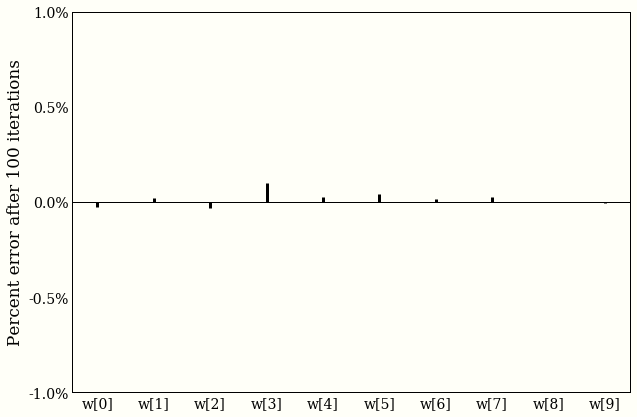
Both our answers agree to within one tenth of one percent, which is exciting, but should not be, because we already did some math.
The jax implementation here requires care in random number generation (and np.linalg.pinv is not yet implemented), so that the GPUs could deal with them. In fact, only the first few lines, and the very last line need to change:
from jax import random

key = random.PRNGKey(1)

data_points, data_dimension = 100, 10

# Generate X and w, then set y = Xw + ϵ
X = random.normal(key, (data_points, data_dimension))

true_w = random.normal(key, (data_dimension,))
y = X.dot(true_w) + 0.1 * random.normal(key, (data_points,))

def make_squared_error(X, y):
    def squared_error(w):
        return np.sum(np.power(X.dot(w) - y, 2)) / X.shape[0]
    return squared_error

# Now use autograd!
grad_loss = grad(make_squared_error(X, y))

# V rough gradient descent routine. don't use this for a real problem.
w_grad = np.zeros(data_dimension)
epsilon = 0.1
iterations = 100
for _ in range(iterations):
    w_grad = w_grad - epsilon * grad_loss(w_grad)

# Linear algebra! The Moore-Penrose pseudoinverse: (X^TX)^{-1}X^T.
w_linalg = np.dot(np.dot(np.linalg.inv(np.dot(X.T, X)), X.T), y)