This is the third post in a series exploring implementing gradient based samplers in practice. The first post is on automatic differentiation, and the second is a basic implementation of Hamiltonian Monte Carlo. A well tested, documented library containing all of this code is available here. Pull requests and issues are welcome.
One of the most immediate improvements you can make to Hamiltonian Monte Carlo (HMC) is to implement step size adaptation, which gives you fewer parameters to tune, and adds in the concept of “warmup” or “tuning” for your sampler. The material here is largely from section 3.2 of Hoffman and Gelman’s The No-U-Turn Sampler: Adaptively Setting Path Lengths in Hamiltonian Monte Carlo.
The acceptance rate
Recall that Hamiltonian Monte Carlo makes a proposal by integrating the Hamiltonian for a set amount of time. We explore the leapfrog integrator more in the next post, but if it worked perfectly, we would always accept the proposal (this should not be obvious!). It does not integrate perfectly though, and we can correct for this using a Metropolis acceptance check. Specifically, with a probability density function $\pi$, starting position and momentum $(\mathbf{q}, \mathbf{p})$ and ending position and momentum $(\mathbf{q}^{\prime}, \mathbf{p}^{\prime})$, we use: $$ P(\text{accept} | (\mathbf{q}, \mathbf{p}), (\mathbf{q}^{\prime}, \mathbf{p}^{\prime})) = \min \left( 1, \frac{\pi(\mathbf{q}^{\prime}, \mathbf{p}^{\prime})}{\pi(\mathbf{q}, \mathbf{p})} \right) $$
In case we do not accept, we add $(\mathbf{q}, \mathbf{p})$ to our samples again, resample the momentum, and make another proposal. In code, this looks like
start_log_p = np.sum(momentum.logpdf(p0)) - negative_log_prob(samples[-1])
new_log_p = np.sum(momentum.logpdf(p_new)) - negative_log_prob(q_new)
p_accept = min(1, np.exp(new_log_p - start_log_p))
if np.random.rand() < p_accept:
    samples.append(q_new)
else:
    samples.append(samples[-1])
This shows how increasing step size decreases the accuracy of the integrator:
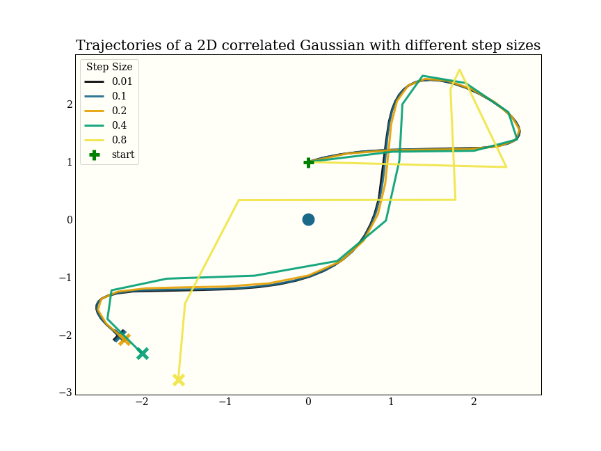
Note that the black line uses 600 gradient evaluations, and ends up in more or less the same spot as the yellow line, which uses only 8 gradient evaluations.
The tradeoff
The dominating cost of doing HMC is the gradient evaluations. See Margossian’s A Review of automatic differentiation and its efficient implementation
for details and careful benchmarks. Here are some naive benchmarks on my laptop, in autograd, for a single evaluation:
| log_pdf | gradient | ratio | |
|---|---|---|---|
| 1d Gaussian | 1.91μs | 127μs | 66.49 |
| 1d Mixture | 60.80μs | 550μs | 9.05 |
| 2d Gaussian | 25.70μs | 267μs | 10.39 |
| 2d Mixture | 165.00μs | 1080μs | 6.55 |
One way to do fewer gradient evaluations is to take bigger steps. This will lower our acceptance rate, but may be worth it. Roughly, we want the fewest gradient evaluations per accepted sample. This experiment was done with a 2d correlated Gaussian:
| step size | samples | accepted | gradients per step | grads/accept |
|---|---|---|---|---|
| 0.05 | 1000 | 1000 | 60 | 60.00 |
| 0.10 | 1000 | 998 | 30 | 30.06 |
| 0.20 | 1000 | 993 | 15 | 15.11 |
| 0.40 | 1000 | 958 | 8 | 8.35 |
| 0.60 | 1000 | 853 | 5 | 5.86 |
| 0.80 | 1000 | 667 | 4 | 6.00 |
| 1.00 | 1000 | 135 | 3 | 22.22 |
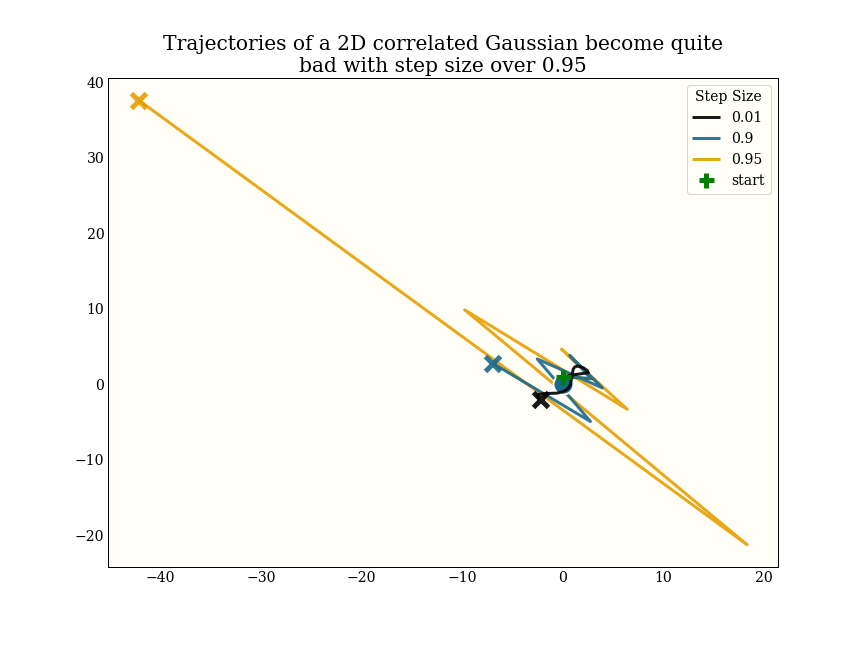
The NUTS paper suggests that an acceptance probability of 0.65 is the optimal balance, and this experiment shows a similar number (66.7% are accepted with a step size of 0.8, which uses around the fewest gradients per acceptance). So how do we automatically choose a step size that accepts around 65% of proposals?
Implementing dual-averaging step size adaptation
Stochastic optimization describes a way to optimize a function in the presence of noise. It is a general algorithm: the algorithm below is from the NUTS paper, but the scheme is based on one from Nesterov’s Primal-dual subgradient methods for convex problems . As a technical note, Nesterov shows how to minimize a convex problem, and here we find the zero of a function. This is like using an algorithm to minimize $f(x) = x^2$ to instead find a zero of $f’(x) = 2x$: we replace the gradient with the accumulated error.
The general idea is to make proposals based on the average error we have seen so far, and dampen the amount of exploration we do over time: our technical requirement is that the proposed log_step is $\mathcal{O}(\sqrt{t})$. At each step, the algorithm will produce a step size used for exploration, and a smoothed version. In practice, we will use the noisy step until we are done tuning, and then fix the smooth (dual-averaged) step size.
We implement this as a class to keep track of some state. There are five parameters supplied, and we use defaults from the NUTS paper (which are also the defaults in PyMC3 and Stan):
initial_step_size: there are ways to automate guessing this, but we do not yet.target_accept: Our goal Metropolis acceptance rategamma: Controls the amount of shrinkage in the exploration stept0: Dampens early exploration: a large value prevents the step size from being huge, which may be very computationally costly.kappa: The smoothed step size is a weighted sum of previous step sizes.kappais a parameter that “forgets” earlier iterates.
class DualAveragingStepSize:
    def __init__(self, initial_step_size, target_accept=0.65, gamma=0.05, t0=10.0, kappa=0.75):
        self.mu = np.log(10 * initial_step_size)  # proposals are biased upwards to stay away from 0.
        self.target_accept = target_accept
        self.gamma = gamma
        self.t = t0
        self.kappa = kappa
        self.error_sum = 0
        self.log_averaged_step = 0

    def update(self, p_accept):
        # Running tally of absolute error. Can be positive or negative. Want to be 0.
        self.error_sum += self.target_accept - p_accept

        # This is the next proposed (log) step size. Note it is biased towards mu.
        log_step = self.mu - self.error_sum / (np.sqrt(self.t) * self.gamma)

        # Forgetting rate. As `t` gets bigger, `eta` gets smaller.
        eta = self.t ** -self.kappa

        # Smoothed average step size
        self.log_averaged_step = eta * log_step + (1 - eta) * self.log_averaged_step

        # This is a stateful update, so t keeps updating
        self.t += 1

        # Return both the noisy step size, and the smoothed step size
        return np.exp(log_step), np.exp(self.log_averaged_step)
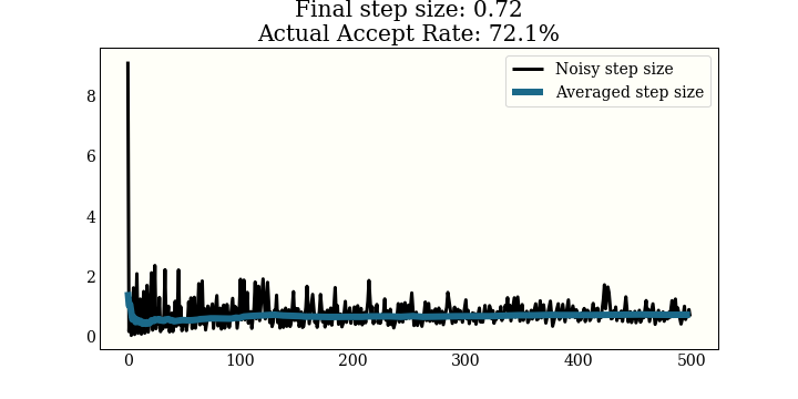
Here is a plot of the noisy step size, along with the smoothed step size over 500 warmup steps. This is run on a 2D Gaussian, trying to get a 65% acceptance rate:
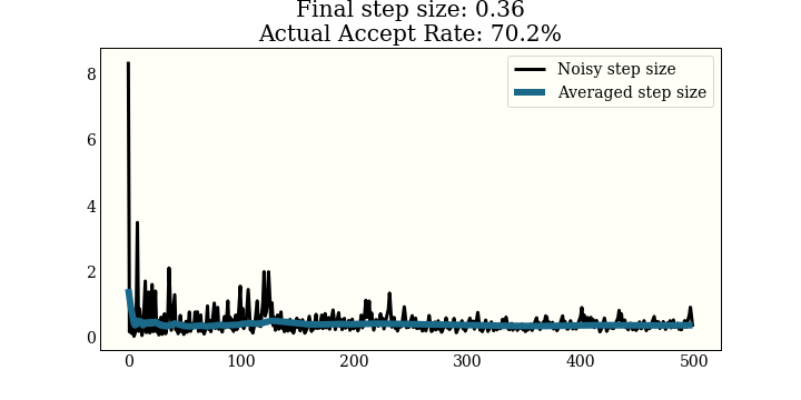
This one is run on a 1D mixture of 3 Gaussians, again with a goal of 65% acceptance
Using the dual averaging step size
To actually use this class, here is code from the previous post implementing basic HMC, but removing extraneous details, and adding dual averaging step size. Note that all we do is add a check to the first ~500 steps, then fix the step size on the 500th:
def hamiltonian_monte_carlo(..., tune=500):
    ...
    step_size_tuning = DualAveragingStepSize(initial_step_size=step_size)
    for idx, p0 in tqdm(enumerate(momentum.rvs(size=size)), total=size[0]):
        q_new, p_new = leapfrog(..., step_size=step_size)
        start_log_p = ...
        new_log_p = ...
        p_accept = min(1, np.exp(new_log_p - start_log_p))
        if np.random.rand() < p_accept:
            samples.append(q_new)
        else:
            samples.append(np.copy(samples[-1]))

        # Tuning routine
        if idx < tune - 1:
            step_size, _ = step_size_tuning.update(p_accept)
        elif idx == tune - 1:
            _, step_size = step_size_tuning.update(p_accept)

    # Throw out tuning samples, as they are not valid MCMC samples
    return np.array(samples[1 + tune :])
Performance changes
Note that if you set the step size perfectly, you have no need for this. In order to really discuss performance here, we would need to discuss and implement:
- Effective sample size Which is, roughly, how many independent samples you produce. MCMC traditionally produces highly correlated samples, and taking long steps increases independence
- Divergence handling When a gradient based sampler fails, it fails catastrophically in a way that is easy to spot. One remedy is to shorten the step size, which corresponds to increasing the desired acceptance rate.
Very roughly, though, I had been using a step size of 0.05 as a default before implementing the step size adaptation, and most of the test distributions I am using adapt to a step size between 0.3 and 0.8, which gives a 6-15x speedup.