This is the second post in a series exploring implementing gradient based samplers in practice. The first post is here. A well tested, documented library containing all of this code is available here. Pull requests and issues are welcome.
The notebook that generated this blog post can be found here.
Markov chain Monte Carlo (MCMC) is a method used for sampling from posterior distributions. Hamiltonian Monte Carlo (HMC) is a variant that uses gradient information to scale better to higher dimensions, and which is used by software like PyMC3 and Stan. Some great references on MCMC in general and HMC in particular are
- Christopher Bishop’s “Pattern Recognition and Machine Learning“ A classic machine learning textbook, and gives a good overview of motivating sampling, as well as a number of different sampling strategies.
- Iain Murray’s lectures at the MLSS A good, approachable lecture, including intuition about how these algorithms are applied and implemented
- Michael Betancourt’s “A Conceptual Introduction to Hamiltonian Monte Carlo“ A thorough, readable reference that is the main source here
Our Strategy
- Give a few pictures of what is going on
- Write down the math we need from Betancourt’s “A Conceptual Introduction to Hamiltonian Monte Carlo”
- Write down the implementation in Python
One thing I am not going to do here is justify why this works: Betancourt and his references do a good job of that. I will mention but not pursue ways to make this algorithm fast, leaving those for future blog posts.
Pictures of what’s going on
Hamiltonian trajectories
Starting from any point, we can generate a new sample from a probability distribution by giving the point some momentum and then updating the position and momentum according to a certain system of differential equations (Hamilton’s equations, whence the name). The differential equation depends on the probability distribution, and we update the position and momentum using “leapfrog integration”. Here are three trajectories of a 2d multivariate normal.
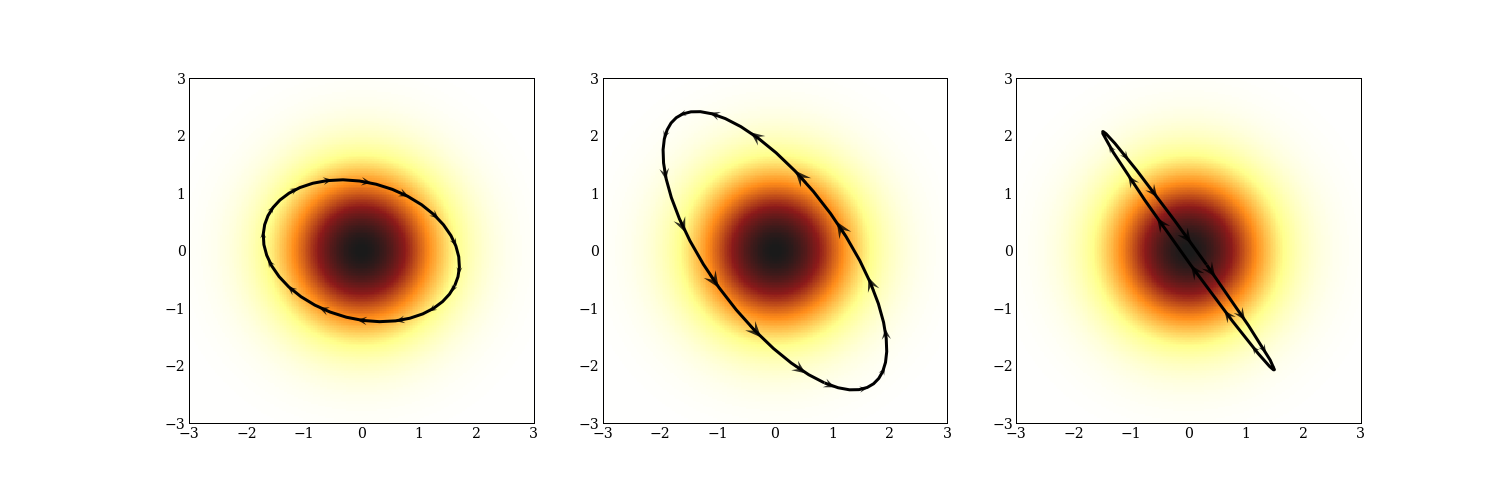
Calculating these trajectories is expensive, and we will do a lot of work to make this less expensive. Sometimes trajectories are not precisely ellipses. Here are three trajectories for a mixture of three normal distributions.
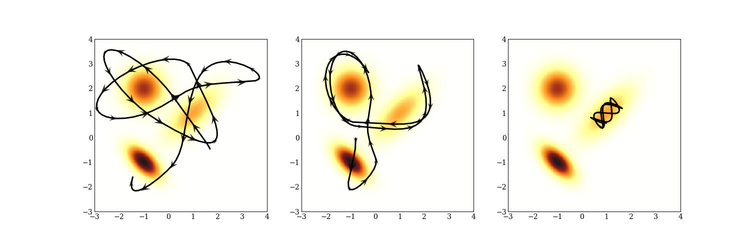
Notice that the Hamiltonian dynamics preserve energy: the momentum is indicated by the size and direction of the arrows; when the trajectory is furthest away from one of the modes, the arrows are very small indicating large potential energy and small kinetic energy. There is also one trajectory that stays very close to a single mode because it does not have the energy to move to another.
There are also tricky probability densities to sample from! One is “Neal’s funnel”, where you draw a normally distributed $\theta$, and then use $e^{\theta}$ as the scale for a normal distribution. This sort of geometry turns up in hierarchical models, and are important to be able to sample from. A benefit of gradient based samplers is that they go very obviously wrong when they go wrong.
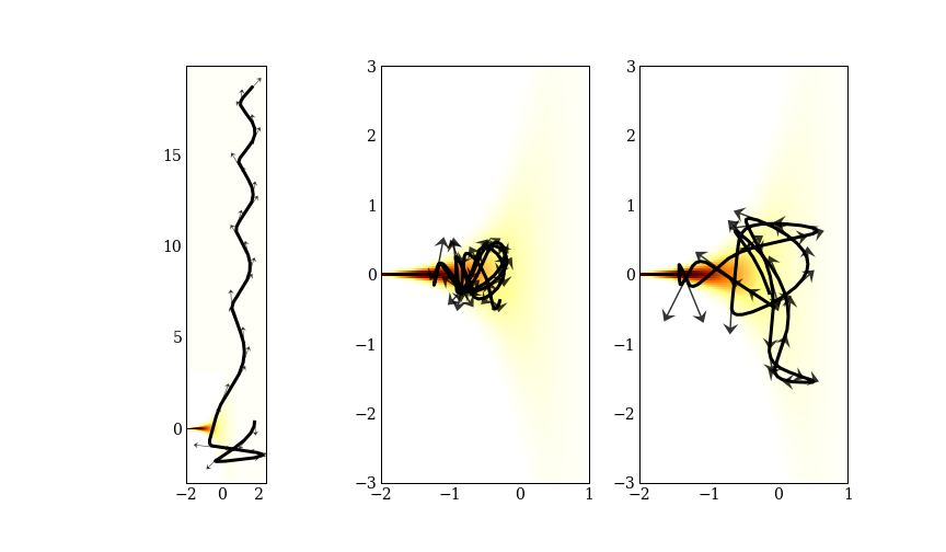
Can you see which of these three trajectories went terribly wrong? We will call these “divergences”, and use them to diagnose problems in a later post.
Hamiltonian Monte Carlo
Once we can generate these Hamiltonian trajectories, we fix an integration length, generate a trajectory of that length, and that is our next sample. Starting from that point, we pick a new momentum at random, and keep going. Here is an example of 10 draws from a 2D multivariate Gaussian with 3 different path lengths.
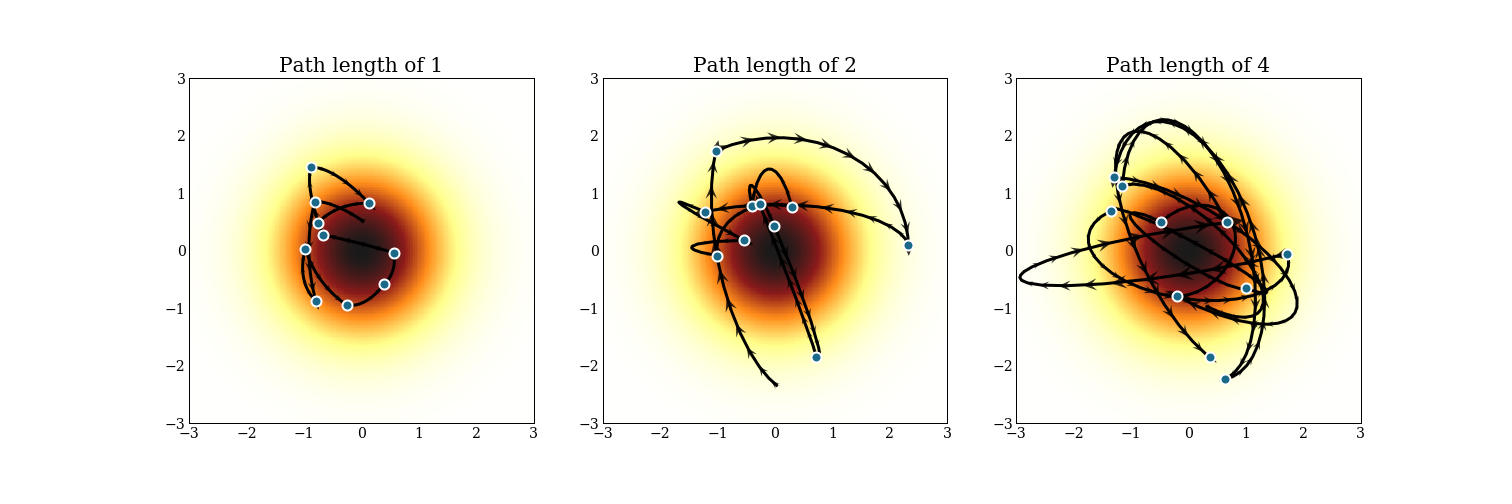
Notice that each trajectory starts from where the previous trajectory ended, but the momentum is totally different. In reality, we will make a much cruder estimate of the trajectory to save computing time, and accept or reject the proposal at the end of the trajectory, usually aiming to accept 60-80% of the time.
Here also are trajectories for a mixture of 3 multivariate normals, again with 3 different path lengths.
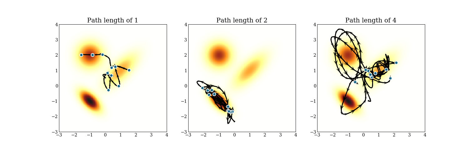
Notice that mixing between modes can be hard, and can take time! The path length of 2 never makes it to a different mode! Of course, this is only drawing 10 samples, but it is something to keep in mind while tuning an HMC sampler.
The math we need for Hamiltonian Monte Carlo
The goal of this section is to present the equations from Betancourt’s paper, so we can reference them in the code.
To reiterate, it should not be obvious why this algorithm samples from the correct distribution. The interested reader will consult one of the references given earlier, particularly Betancourt’s paper, whose notation I will use.
How HMC works
- We concatenate all of our parameters into a single position variable, $\mathbf{q}$. We are trying to sample from the probability density function $\pi(\mathbf{q})$.
- We add a momentum variable, $\mathbf{p}$, of the same dimension as $\mathbf{q}$, and consider the probability distribution $$ \pi(\mathbf{q}, \mathbf{p}) = \pi(\mathbf{p} | \mathbf{q}) \pi(\mathbf{q}), $$ where we get to choose $\pi(\mathbf{p} | \mathbf{q})$. In practice, we will choose $\pi(\mathbf{p} | \mathbf{q}) = \mathcal{N}(\mathbf{0}, M)$, and in this essay, we will choose $M = I$.
- Define the Hamiltonian, $H(\mathbf{q}, \mathbf{p}) = -\log \pi(\mathbf{q}, \mathbf{p})$.Given the factorization above, we get $$ H(\mathbf{q}, \mathbf{p}) = -\log \pi(\mathbf{p} | \mathbf{q}) - \log \pi(\mathbf{q}) = K(\mathbf{p}, \mathbf{q}) + V(\mathbf{q}), $$ where $K(\mathbf{p}, \mathbf{q})$ is called the kinetic energy, and $V(\mathbf{q})$ is called the potential energy, using an analogy to physical systems.
- We evolve the system $(\mathbf{q}, \mathbf{p})$ according to Hamilton’s equations:
$$
\frac{d \mathbf{q}}{dt} = \frac{\partial H}{\partial \mathbf{p}} = \frac{\partial K}{\partial \mathbf{p}} + \frac{\partial V}{\partial \mathbf{p}}\\
\frac{d \mathbf{p}}{dt} = -\frac{\partial H}{\partial \mathbf{q}}= -\frac{\partial K}{\partial \mathbf{q}} - \frac{\partial V}{\partial \mathbf{q}} $$ Note that $\frac{\partial V}{\partial \mathbf{p}} = \mathbf{0}$.
We chose the kinetic energy to be a Gaussian, which lets us calculate those gradients by hand instead of recalculating them. Specifically, $$ K(\mathbf{p}, \mathbf{q}) = \frac{1}{2}\mathbf{p}^T M^{-1}\mathbf{p} + \log |M| + \text{const.}, $$ and with our choice of $M = I$, $$ K(\mathbf{p}, \mathbf{q}) = \frac{1}{2}\mathbf{p}^T \mathbf{p} + \text{const.}, $$ so $$ \frac{\partial K}{\partial \mathbf{p}} = \mathbf{p} $$ and $$ \frac{\partial K}{\partial \mathbf{q}} = \mathbf{0} $$
We can then simplify Hamilton’s equations to:
$$
\frac{d \mathbf{q}}{dt} = \mathbf{p} \\
\frac{d \mathbf{p}}{dt} = - \frac{\partial V}{\partial \mathbf{q}}
$$
This is the algorithm, then: - Sample a $\mathbf{p} \sim \mathcal{N}(0, I)$, - Simulate $\mathbf{q}(t)$ and $\mathbf{p}(t)$ for some amount of time $T$ using the simplified equations above - $\mathbf{q}(T)$ is our new sample.
Hamiltonian Monte Carlo in code
This is a small function. A few things to notice in particular:
- We need to compute $\frac{\partial V}{\partial \mathbf{q}}$, and do so using autodiff. See my previous post on autodiff libraries. The
negative_log_probargument must be defined usingautograd. - We still need to define the function
leapfrog, which is below. - There is a Metropolis acceptance dance at the bottom. This corrects for errors introduced by the
leapfrogintegrator. I had a bug in this implementation that was hard to spot: we are sampling from $\pi(\mathbf{q}, \mathbf{p})$ here, not $\pi(\mathbf{q})$, so the momentum at the end of the trajectory needs to be returned by the leapfrog function, too.
from autograd import grad
import autograd.numpy as np
import scipy.stats as st


def hamiltonian_monte_carlo(n_samples, negative_log_prob, initial_position, path_len=1, step_size=0.5):
    """Run Hamiltonian Monte Carlo sampling.

    Parameters
    ----------
    n_samples : int
        Number of samples to return
    negative_log_prob : callable
        The negative log probability to sample from
    initial_position : np.array
        A place to start sampling from.
    path_len : float
        How long each integration path is. Smaller is faster and more correlated.
    step_size : float
        How long each integration step is. Smaller is slower and more accurate.

    Returns
    -------
    np.array
        Array of length `n_samples`.
    """
    # autograd magic
    dVdq = grad(negative_log_prob)

    # collect all our samples in a list
    samples = [initial_position]

    # Keep a single object for momentum resampling
    momentum = st.norm(0, 1)

    # If initial_position is a 10d vector and n_samples is 100, we want
    # 100 x 10 momentum draws. We can do this in one call to momentum.rvs, and
    # iterate over rows
    size = (n_samples,) + initial_position.shape[:1]
    for p0 in momentum.rvs(size=size):
        # Integrate over our path to get a new position and momentum
        q_new, p_new = leapfrog(
            samples[-1],
            p0,
            dVdq,
            path_len=path_len,
            step_size=step_size,
        )

        # Check Metropolis acceptance criterion
        start_log_p = negative_log_prob(samples[-1]) - np.sum(momentum.logpdf(p0))
        new_log_p = negative_log_prob(q_new) - np.sum(momentum.logpdf(p_new))
        if np.log(np.random.rand()) < start_log_p - new_log_p:
            samples.append(q_new)
        else:
            samples.append(np.copy(samples[-1]))

    return np.array(samples[1:])
The Leapfrog Integrator
How do we simulate the differential equations above? A natural approach is to discretize t, and go back and forth updating q and p. It turns out this causes errors to accumulate in systematic ways, but there is a nice algorithm to simulate Hamiltonian dynamics. It involves updating the momentum p a half step, then the position q a whole step, and then finish updating p the other half of the step. When you do this in a loop, most of the half-step updates combine, and you just have to do some book-keeping at either end. There is also a momentum flip at the end that is important for technical reasons.
def leapfrog(q, p, dVdq, path_len, step_size):
    """Leapfrog integrator for Hamiltonian Monte Carlo.

    Parameters
    ----------
    q : np.floatX
        Initial position
    p : np.floatX
        Initial momentum
    dVdq : callable
        Gradient of the velocity
    path_len : float
        How long to integrate for
    step_size : float
        How long each integration step should be

    Returns
    -------
    q, p : np.floatX, np.floatX
        New position and momentum
    """
    q, p = np.copy(q), np.copy(p)

    p -= step_size * dVdq(q) / 2  # half step
    for _ in range(int(path_len / step_size) - 1):
        q += step_size * p  # whole step
        p -= step_size * dVdq(q)  # whole step
    q += step_size * p  # whole step
    p -= step_size * dVdq(q) / 2  # half step

    # momentum flip at end
    return q, -p