PyMC3 v3.8
Released 29 November, 2019
See PyMC3 on GitHub here, the docs here, and the release notes here. This post is available as a notebook here.
This is my own work, so apologies to the contributors for my failures in summing up their contributions, and please direct mistakes my way. Thanks also to all the contributors for the bug fixes, maintenance, code reviews, issue reporting, and so on that went into this release. I actually tried to not call out individual authors here, since open source is such a collaborative effort.
import pymc3 as pm
import numpy as np
from scipy.integrate import odeint
import matplotlib.pyplot as plt


print(pm.__version__)
3.8
Implemented robust u turn check in NUTS (similar to stan-dev/stan#2800) #3605.
This was a technical improvement on PyMC3’s core algorithm, the No-U-Turn sampler (NUTS), probably best explained in the Stan discourse page.
Roughly, NUTS is distinguished from Hamiltonian Monte Carlo (HMC) in that it can explore posterior distributions of different scales using a dynamic path length. HMC, by contrast, will have a fixed path length. Longer paths will be slower, but produce “more independent” samples. NUTS uses a heuristic to balances these desires: when the trajectory “makes a U-turn”, we stop integrating.
User nhuurre found that this U-turn check was not actually catching all the U-turns, and the Stan development team was able to reproduce that this could and did actually occur, and that it was a technical, but not onerous, fix. End users do not need to do anything to opt into this feature (in fact, you can’t opt out), but it is worth pointing out that this correction is implemented.
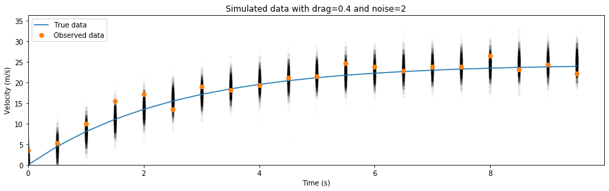
Add capabilities to do inference on parameters in a differential equation with DifferentialEquation. See #3590 and #3634.
This was completed as part of GSoC. See Demetri’s post on the work for a better description.
Below is an example ODE, modelling an object in free fall under the effects of drag. We will try to estimate the drag coefficient under some uncertain observations.
np.random.seed(0)

def freefall(drag, t, velocity):
    """Equation for an object falling under the force of gravity.

    y' = mg - γy

    where y is velocity, m is the mass (we set to 1.), γ is drag, g is gravity (9.8 m/s^2).
    """
    return 9.8 - velocity[0] * drag[0]


# Generate fake data
# Unobserved parameters are suffixed with "_", like "drag_"
times = np.arange(0, 10, 0.5)
drag_, sigma_ = 0.4, 2
y_ = odeint(freefall, t=times, y0=0., args=tuple([[drag_]]))
y_obs = np.random.normal(y_, sigma_)

ode_model = pm.ode.DifferentialEquation(
    func=freefall,
    times=times,
    n_states=1,
    n_theta=1,
    t0=0)

with pm.Model():
    sigma = pm.HalfCauchy('sigma', 1)
    drag = pm.Lognormal('drag', 0, 1)
    ode_solution = ode_model(y0=[0], theta=[drag])
    Y = pm.Normal('Y', mu=ode_solution, sd=sigma, observed=y_obs)

    trace = pm.sample(500, tune=1000)
    ppc = pm.sample_posterior_predictive(trace)
Auto-assigning NUTS sampler...
Initializing NUTS using jitter+adapt_diag...
Multiprocess sampling (4 chains in 4 jobs)
NUTS: [drag, sigma]
Sampling 4 chains, 0 divergences: 100%|██████████| 6000/6000 [01:58<00:00, 50.81draws/s]
100%|██████████| 2000/2000 [00:24<00:00, 81.56it/s]
The posterior for sigma and drag are calculated in the presence of noise, and we can plot the posterior predictive samples on top of the original dataset to see what might have happened if we reran the experiment using these posterior estimates:
Distinguish between Data and Deterministic variables when graphing models with graphviz. PR #3491.
This is a quality-of-life improvement on how the model_to_graphviz function draws a model. This PR added rounded corners to the Data node to distinguish it from a Deterministic, and also added an octagon for a Potential node.
with pm.Model() as model:
    x = pm.Normal('x')
    y = pm.Deterministic('y', np.abs(x))
    pm.Potential('z', pm.Normal.dist().logp(x))
    observation = pm.Data('my_observation', [1, 2, 0])
    pm.Normal('observed', mu=x, sd=y, observed=observation)

pm.model_to_graphviz(model)

Sequential Monte Carlo - Approximate Bayesian Computation step method is now available. The implementation is in an experimental stage and will be further improved.
This is also known as likelihood-free inference. This provides a Simulator and a sample_smc method, and compares the simulated data with your observed data. Note also the warning when you use these functions!
data = np.random.randn(1000)

def normal_sim(a, b):
    return np.sort(np.random.normal(a, b, 1000))


with pm.Model():
    a = pm.Normal('a', mu=0, sd=5)
    b = pm.HalfNormal('b', sd=1)
    s = pm.Simulator('s', normal_sim, observed=np.sort(data))
    trace_example = pm.sample_smc(kernel="ABC", epsilon=0.1)

pm.summary(trace_example)
Sample initial stage: ...
/home/colin/projects/pymc3/pymc3/smc/smc.py:120: UserWarning: Warning: SMC-ABC methods are experimental step methods and not yet recommended for use in PyMC3!
  warnings.warn(EXPERIMENTAL_WARNING)
Stage:   0 Beta: 0.002 Steps:  25 Acce: 1.000
Stage:   1 Beta: 0.019 Steps:  25 Acce: 0.514
Stage:   2 Beta: 0.096 Steps:   6 Acce: 0.441
Stage:   3 Beta: 0.328 Steps:   7 Acce: 0.343
Stage:   4 Beta: 1.000 Steps:  10 Acce: 0.332
| mean | sd | hpd_3% | hpd_97% | mcse_mean | mcse_sd | ess_mean | ess_sd | ess_bulk | ess_tail | r_hat | |
|---|---|---|---|---|---|---|---|---|---|---|---|
| a | -0.017 | 0.114 | -0.242 | 0.176 | 0.004 | 0.003 | 911.0 | 911.0 | 919.0 | 981.0 | NaN |
| b | 0.988 | 0.127 | 0.739 | 1.215 | 0.004 | 0.003 | 963.0 | 963.0 | 964.0 | 906.0 | NaN |
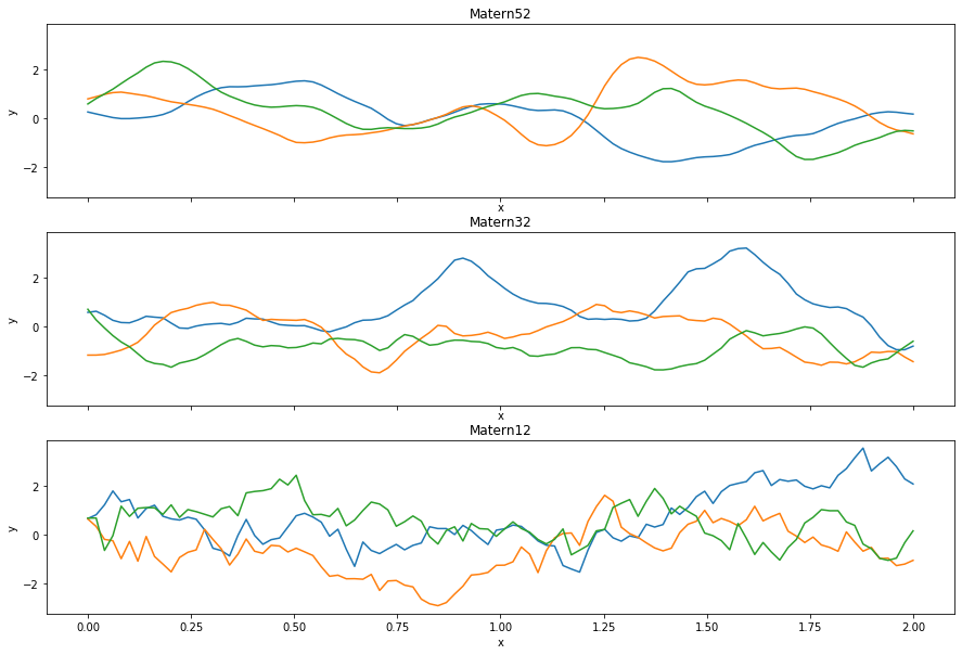
Added Matern12 covariance function for Gaussian processes. This is the Matern kernel with nu=1⁄2.
The Matern kernels are parameterized by $\nu$, and are generalizations of the radial basis function (RBF) kernel. They are computationally pleasant for $\nu = \infty$, which recovers the RBF kernel, $\nu = 5 / 2 $, which are twice differentiable functions, $\nu = 3 / 2$, differentiable functions, and $\nu = 1 / 2$, which is the absolute exponential kernel. PyMC3 already implemented Matern52 and Matern32, so Matern12 completes the set. You can see comparisons below:
Progressbar reports number of divergences in real time, when available #3547.
This is helpful for long running models: if you have tons of divergences, maybe you want to quit early and think about what you have done. Below is a model that most samplers have trouble with (Neal’s funnel). This feature adds the Sampling 4 chains, $N divergences text. Note that after the sampling is done, each chain reports problems separately!
with pm.Model() as funnel:
    scale = pm.Normal("scale", mu=0, sd=3)
    pm.Normal("x", sd=pm.math.exp(scale / 2), shape=10)
    trace = pm.sample()
Auto-assigning NUTS sampler...
Initializing NUTS using jitter+adapt_diag...
Multiprocess sampling (4 chains in 4 jobs)
NUTS: [x, scale]
Sampling 4 chains, 5 divergences: 100%|██████████| 4000/4000 [00:05<00:00, 705.25draws/s]
There was 1 divergence after tuning. Increase `target_accept` or reparameterize.
The acceptance probability does not match the target. It is 0.5371405758649728, but should be close to 0.8. Try to increase the number of tuning steps.
There was 1 divergence after tuning. Increase `target_accept` or reparameterize.
There were 3 divergences after tuning. Increase `target_accept` or reparameterize.
The acceptance probability does not match the target. It is 0.46186288892493643, but should be close to 0.8. Try to increase the number of tuning steps.
The rhat statistic is larger than 1.05 for some parameters. This indicates slight problems during sampling.
The estimated number of effective samples is smaller than 200 for some parameters.
Sampling from variational approximation now allows for alternative trace backends #3550.
This is also something you can already do with inference, though alternative backends are not well supported (pull requests always welcome!), and now it works with variational inference as well.
import pandas as pd
import sqlite3

with pm.Model():
    pm.Normal('x')

    fit = pm.fit()
    trace = fit.sample(backend='sqlite', name='trace.db')

db = sqlite3.connect('trace.db')
pd.read_sql('SELECT * FROM x', db, index_col='recid').head()
Average Loss = 0.0024892: 100%|██████████| 10000/10000 [00:02<00:00, 3522.38it/s]
Finished [100%]: Average Loss = 0.0025052
| draw | chain | v | |
|---|---|---|---|
| recid | |||
| 1 | 0 | 0 | 0.249017 |
| 2 | 1 | 0 | -2.217926 |
| 3 | 2 | 0 | -0.489882 |
| 4 | 3 | 0 | -1.458609 |
| 5 | 4 | 0 | 0.977264 |
Infix @ operator now works with random variables and deterministics #3619.
Another quality of life improvement. This uses the matrix multiplication operator that has been available since Python 3.5.
X = np.random.randn(100, 1)
w = np.random.randn(1)
y = X @ w + (np.random.randn(100) * .1)

with pm.Model() as linear_model:
    weights = pm.Normal('weights', mu=0, sigma=1)
    noise = pm.Gamma('noise', alpha=2, beta=1)
    y_observed = pm.Normal('y_observed',
                           mu=X @ weights,  # hooray!
                           sigma=noise,
                           observed=y)
ArviZ is now a requirement, and handles plotting, diagnostics, and statistical checks.
Check out the ArviZ docs, and file issues as they come up. This transition might be at least a little bumpy, but it unifies efforts between a number of different probabilistic programming libraries, and makes sure that calculations like effective sample size are consistent between these different libraries.
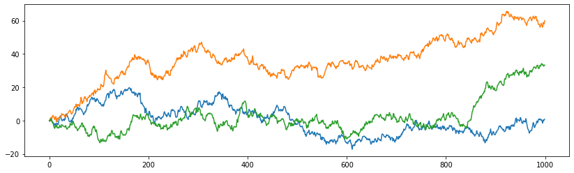
Can use GaussianRandomWalk in sample_prior_predictive and sample_prior_predictive #3682.
There has been considerable work over the past year in allowing prior predictive and posterior predictive sampling, and this starts implementing these methods for the GaussianRandomWalk. This allowed the stochastic volatility example to be rewritten and including a prior- and posterior-predictive check.
Here we are just using the .random() method directly to generate 3 series of length 1,000:
fig, ax = plt.subplots(figsize=(14, 4))
ax.plot(pm.GaussianRandomWalk.dist(shape=(1000, 3)).random());
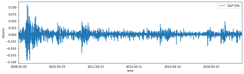
Now 11 years of S&P returns in data set #3682.
Again in service of the stochastic volatility example, PyMC3 ships with 11 years of data!
returns = pd.read_csv(pm.get_data("SP500.csv"), index_col='Date')
returns["change"] = np.log(returns["Close"]).diff()
returns = returns.dropna()

fig, ax = plt.subplots(figsize=(14, 4))
returns.plot(y="change", label='S&P 500', ax=ax)
ax.set(xlabel='time', ylabel='returns')
ax.legend();