“Four chains isn’t cool. You know what’s cool? A million chains.”
I have been spending a lot of time with TensorFlow Probability in the last year in working on PyMC4 and generally doing Bayesian things. One feature that I have not seen emphasized - but I find very cool - is that chains are practically free, meaning running hundreds or thousands of chains is about as expensive as running 1 or 4.
What is a chain?
A chain is an independent run of MCMC. Running multiple chains can help diagnose multimodality (as in the linked answer), and allows for convergence diagnostics.
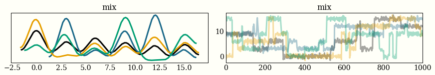
Sampling from a mixture of six Gaussians using four chains looks pretty funny. The left plot is a histogram from each of the four chains, and the right is a timeseries of the 1,000 draws for each of the chains. I say this looks funny because you can see the chains jumping from one mode to the next, so you might conclude that you have not spent enough time in each mode, or even found all of them.
How are chains usually implemented?
I have always seen libraries
- Implement an MCMC sampler, and then
- Use some sort of multiprocessing library to repeat it multiple times.
For example, PyMC3 used to use joblib, and now uses a custom implementation. So if you have 4 cores, you will run 4 independent chains in about the same amount of time as a single chain, or 100 independent chains in ~25x the amount of time as a single chain.
By default, PyMC3 will run one chain for each core available. This used 4 cores to sample 4 chains, and did it in less than a second.
What are we impressed by again?
The above is pretty nice, but maybe we can do better. If you write an algorithm for “MCMC with multiple chains” as a vectorized routine, then instead of running your algorithm for “MCMC” multiple times, you can run “MCMC with multiple chains” once. Hopefully the linear algebra you used gives you performance gains, too.
In a very hand-wavy way, we go from
usual_version = [run_mcmc(iters) for _ in range(chains)]
to
vectorized_version = run_mcmc(iters, chains)
What can we do with thousands of chains?
I am actually not sure! My impression is that there is low-hanging fruit here, but there are a couple places I have seen or found thousands of chains to be useful.
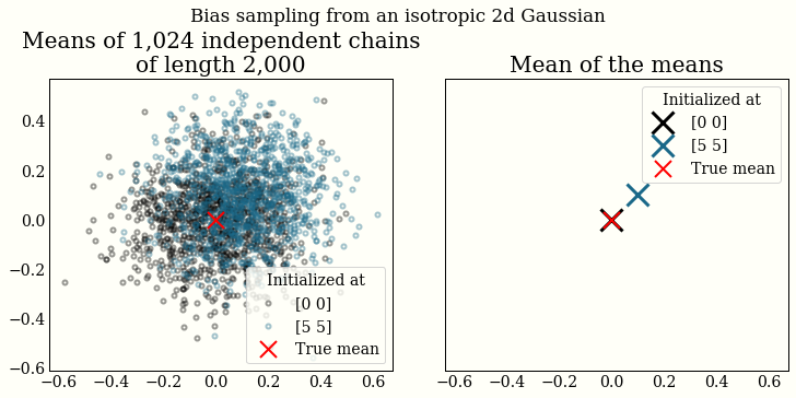
I have been playing with unbiased MCMC with couplings recently. What does it mean for MCMC to be unbiased? Recall that MCMC is only asymptotically from the stationary distribution, so if a chain is not initialized properly, the mean will be biased (discarding some burn-in/warmup draws helps). We can see this by plotting the mean of thousands of (finite-length) chains:
In the very interesting NeuTra-Lizing Bad Geometry in Hamiltonian Monte Carlo Using Neural Transport, the authors use thousands of chains in the experiments to report estimates of the algorithm’s performance:
For all HMC experiments we used the corresponding q(θ) as the initial distribution. In all cases, we ran the 16384 chains for 1000 steps to compute the bias and chain diagnostics, and ran with 4096 chains to compute steps/second.
It seems like there is something useful to be done with tuning MCMC algorithms. For example, step size adaptation is a one dimensional stochastic optimization problem, and may be able to be “solved” with grid search: choose a heuristic upper and lower bound on the step size, run a few iterations with step size
tf.linspace(lower, upper, num_chains), and then choose the optimal step size.
How can I use thousands of chains?
TensorFlow Probability Here is a gist showing how to run Hamiltonian Monte Carlo in TensorFlow Probability with 256 chains.
Numpy I have included a complete numpy implementation of a Metropolis-Hastings sampler at the end of this post, to give a taste of what it looks like (it is about 20 lines of code).
How free is it?
In each experiment, I took 1,000 samples from a standard Gaussian using 4 chains, and from 1,024 chains. This means 256 times as many samples.
TensorFlow Probability was using Hamiltonian Monte Carlo, and took 18.2 seconds vs 22.4 seconds (1.2x as long). I have done some experiments where this is ~10x faster with XLA compilation.
Numpy Implementation is below, and uses Metropolis-Hastings, so we expect it to be faster. It took 17.5ms vs 152ms (8.7x as long).
In Conclusion
Keep an eye out for massive numbers of chains, or for ways to use lots of chains. I think there is some interesting work to do here!
Numpy Implementation
import numpy as np

def metropolis_hastings_vec(log_prob, proposal_cov, iters, chains, init):
    """Vectorized Metropolis-Hastings.

    Allows pretty ridiculous scaling across chains:
    Runs 1,000 chains of 1,000 iterations each on a
    correlated 100D normal in ~5 seconds.
    """
    proposal_cov = np.atleast_2d(proposal_cov)
    dim = proposal_cov.shape[0]
    # Initialize with a single point, or an array of shape (chains, dim)
    if init.shape == (dim,):
        init = np.tile(init, (chains, 1))

    samples = np.empty((iters, chains, dim))
    samples[0] = init
    current_log_prob = log_prob(init)

    proposals = np.random.multivariate_normal(np.zeros(dim), proposal_cov,
                                              size=(iters - 1, chains))
    log_unifs = np.log(np.random.rand(iters - 1, chains))
    for idx, (sample, log_unif) in enumerate(zip(proposals, log_unifs), 1):
        proposal = sample + samples[idx - 1]
        proposal_log_prob = log_prob(proposal)
        accept = (log_unif < proposal_log_prob - current_log_prob)

        # copy previous row, update accepted indexes
        samples[idx] = samples[idx - 1]
        samples[idx][accept] = proposal[accept]

        # update log probability
        current_log_prob[accept] = proposal_log_prob[accept]
    return samples
You can use this sampler with, for example,
import scipy.stats as st

dim = 10
Σ = 0.1 * np.eye(dim) + 0.9 * np.ones((dim, dim))

# Correlated Gaussian
log_prob = st.multivariate_normal(np.zeros(dim),  Σ).logpdf

proposal_cov = np.eye(dim)
iters = 2_000
chains= 1_024
init = np.zeros(dim)

samples = metropolis_hastings_vec(log_prob, proposal_cov, iters, chains, init)