This pageg is available as a colaboratory notebook, and this post has edited out some of the matplotlib code for readability, while retaining the TensorFlow 2.0 code for novelty.
These are notes from a PyMC journal club on January 18, 2019, in preparation for reading Michael Betancourt’s new article on A Geometric Theory of Higher-Order Automatic Differentiation, which makes extensive use of differential geometry. These notes are essentially an elaboration of chapter 0, section 1-3 in Manfredo do Carmo’s Riemannian Geometry.
This is pretty long! Your best bet might be to get the book, read through the first ~10 pages, then refer to this notebook. You might also view the notebook as an example of using TensorFlow 2.0, and some matplotlib functions - I learned about plt.quiver and that the 3d plotting is pretty easy now.
Big Picture
- We can calculate derivatives of functions from $\mathbb{R}^n \rightarrow \mathbb{R}^m$, using calculus
- If we have a real-valued function on some set with nice properties (a smooth manifold), we can still do a lot of calculus
- We do our calculations using a parameterization, and are interested in what happens when we change that parameterization
Function composition
A lot of what we will do is “pushing” functions, also called function composition. That is, if $f : A \rightarrow B$ and $g: B \rightarrow C$, then $g \circ f : A \rightarrow C$.
I try to provide working code examples for a lot of the concepts. For an example of function composition, consider:
def powers(t):
    """Function from R -> R^4"""
    return [t ** j for j in range(4)]

def my_sum(*elements):
    """Function from R^n -> R"""
    return sum(elements)

def composition(t):
    """Function from R -> R"""
    return my_sum(*powers(t))

print(powers(2))
print(my_sum(*powers(2)))
print(composition(2))
[1, 2, 4, 8]
15
15
Review of calculus
We start by remembering derivatives and gradients from calculus, and showing how to perform and visualize these calculations using TensorFlow and matplotlib. We are limited to 3 dimensions for visualization, so we will look at functions
- $\mathbb{R} \rightarrow \mathbb{R}$
- $\mathbb{R} \rightarrow \mathbb{R}^2$
and consider what gradients mean in each of these places.
Functions $\mathbb{R} \rightarrow \mathbb{R}$
These are usually covered in single variable calculus, and allow you to miss some of the “vector”-y stuff that happens in higher dimensions. In particular, I will plot the derivative as a bunch of tangent arrows on the function, rather than as a separate graph, to emphasize that the gradient is a vector at a point.
t = tf.linspace(-2 * np.pi, 2  * np.pi, 100)

with tf.GradientTape() as g:
    g.watch(t)
    f = tf.cos(t)
grad = g.gradient(f, t)
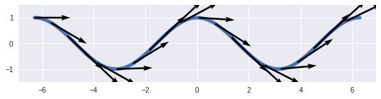
Notice that the gradient is the derivative, and is a function from $\mathbb{R} \rightarrow \mathbb{R}$, $(\cos)`(t) = -\sin t$.
Functions $\mathbb{R} \rightarrow \mathbb{R}^2$
These are parametric curves, $$ f(t) = (x(t), y(t)) $$ and now our gradient will be the element-wise gradient, $$ f’(t) = (x’(t), y’(t)) $$
t = tf.linspace(0., 2 * np.pi, 50)

# `persistent=True` because we extract two gradients here
with tf.GradientTape(persistent=True) as g:
    g.watch(t)
    f = [tf.cos(t), tf.sin(t)]

# Note: `g.gradient(f, t)` returns `sum(grads)`
grads = [g.gradient(func, t) for func in f]
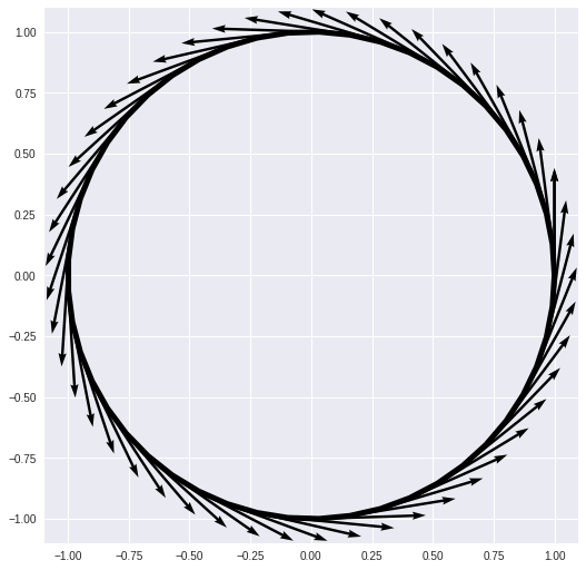
Notice that the gradient is a function from $[0, 2 \pi] \rightarrow \mathbb{R}^2$:
$$ f’(t) = (-\sin t, \cos t) $$
Surfaces
I pick up now with Chapter 0 of do Carmo’s Differential Geometry. The fact that I am emphasizing here is that:
In calculus, we prove that a change of parameters is differentiable. In differential geometry, that is part of the definition.
In order to emphasize this, we should consider:
- What does a change of parameters even mean?
- What does it mean to be differentiable?
Functions $\mathbb{R}^2 \rightarrow \mathbb{R}$
First we need to define nice, invertible functions:
Definition (homeomorphism) A function $\mathbf{x}$ is a homeomorphism if
- $\mathbf{x}$ is 1-to-1 and onto
- $\mathbf{x}$ is continuous
- $\mathbf{x}^{-1}$ is continuous
Discussion In most examples I have seen, we define the range of a map to be wherever it maps, so it is mechanically a surjective (onto) mapping. So if we want to make our parametric map of the circle above into a homeomorphism, we are mostly doing bookkeeping of domains and ranges:
Consider
$$ \mathbf{x}: \mathbb{R} \rightarrow \mathbb{R}^2 = (\cos t, \sin t) $$
Note that this is not injective (1-to-1), since $\mathbf{x}(0) = \mathbf{x}(2 \pi) = (1, 0)$. It is also not surjective (onto), since no value of $t$ maps to $(0, 0) \in \mathbb{R}^2$.
Then we instead define $$ \mathbf{x}: [0, 2 \pi) \rightarrow {\mathbf{x}(t) \in \mathbb{R}^2: t \in [0, 2 \pi)} = (\cos t, \sin t) $$
Now this is 1-to-1, onto, and continuous, and has an inverse for each point on the circle:
$$ \mathbf{x}^{-1}(x_1, x_2) = \arctan \frac{x_1}{x_2} + \frac{\pi}{2}, $$
where we would do some bookkeeping for $x_2 = 0$ and making sure $\arctan$ mapped to $[0, 2 \pi)$.
Now we can provide do Carmo’s definition of a regular surface:
Definition (regular surface) $S \subset \mathbb{R}^3$ is a regular surface if, for every $p \in S$, there exists a neighborhood $V$ of $p$ and $\mathbf{x} : U \subset \mathbb{R}^2 \rightarrow V \cap S$ so that
- $\mathbf{x}$ is a differentiable homeomorphism
- The differential $(d\mathbf{x})_q : \mathbb{R}^2 \rightarrow \mathbb{R}^3$ is injective for all $q \in U$.
Discussion This definition defines a surface as a subset of $\mathbb{R}^3$ as being a surface: the map $\mathbf{x}$ is not the surface! It is important, and will be part of the definition of a manifold, that there are many different maps that give the same surface.
Note that the differential $(d \mathbf{x})_q$ is a $3\times 2$ matrix, and injectivity means that is has full rank. The discussion of neighborhoods above should remind you of the discussion about homeomorphisms above (bookkeeping so the maps are 1-to-1 and onto), and continuity conditions for those familiar with topology (this connection will not be needed to understand the rest of this).
Let’s look at an example of a surface to motivate a concrete discussion:
X, Y = tf.meshgrid(tf.linspace(-2., 2., 50), tf.linspace(-2., 2., 50))
hyperbolic_parabaloid = lambda x, y: 1 - x**2 + y**2 # look it up

with tf.GradientTape() as g:
    g.watch([X, Y])
    f = hyperbolic_parabaloid(X, Y)

grad = g.gradient(f, [X, Y])
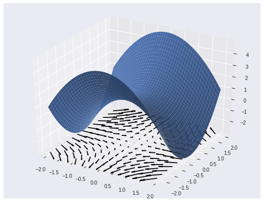
If we claim the thing plotted above is a regular surface, we need to show every point has a neighborhood that is the image of a differentiable homeomorphism with an injective differential. Phew!
Luckily, we claim that all points have the same neighborhood and the same differentiable homeomorphism. Specifically, the set $U \subset \mathbb{R}^2$ is $(-2, 2) \times (-2, 2)$, and in the code, we generate this with tf.meshgrid. Also, the map $\mathbf{x}: U \rightarrow S$ is the function hyperbolic_parabaloid, given by
$$ \mathbf{x}(x_1, x_2) = (x_1, x_2, 1 - x_1^2 + x_2^2), $$
which is continuous, because polynomials are. The differential is given by
$$
(d\mathbf{x})_{(x_1, x_2)} = \begin{bmatrix}
1 & 0
0 & 1
-2x_1 & 2x_2
\end{bmatrix}
$$
The fact that it exists and is continuous means that $\mathbf{x}$ is differentiable, and it has rank 2 (i.e., full rank, i.e., “is injective”) for any $(x_1, x_2)$ because the columns are independent.
We still need to show that the inverse is continuous. But the inverse is so silly it feels like cheating, and is given by
$$ \mathbf{x}^{-1}(y_1, y_2, y_3) = (y_1, y_2) $$
In words: just project the surface onto the plane to get the inverse.
Definition (parameterization) A map $\mathbf{x}$ that defines a regular surface $S$ in a neighborhood of $p \in S$ is called a parameterization of $S$ at $p$.
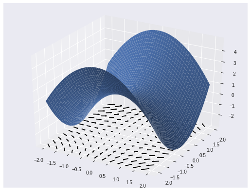
Discussion Note that in the definition of a regular surface, $S$ did not care about $U$. So we can trivially write down another parameterization of the exact same surface $S$, but with $U = (-4, 4) \times (-4, 4)$.
X, Y = tf.meshgrid(tf.linspace(-4., 4., 50), tf.linspace(-4., 4., 50))
hyperbolic_parabaloid_param2 = lambda x, y: 1 - (x / 2)**2 + (y / 2)**2 # look it up

with tf.GradientTape() as g:
    g.watch([X, Y])
    f = hyperbolic_parabaloid_param2(X, Y)

grad = g.gradient(f, [X, Y])
The highlight of multivariable differentiable calculus
Just like a homeomorphism is a continuous function with continuous inverse, a diffeomorphism is a differentiable function with differentiable inverse. do Carmo in fact assumes smoothness, so the function and its inverse have infinitely many derivatives.
Theorem (important) A change of parameters is a diffeomorphism.
This will be part of the definition of a manifold, but it is a theorem that is proved in a calculus course. We haven’t defined a change of parameters yet!
Definition (change of parameters) If $\mathbf{x}_{\alpha} : U_{\alpha} \rightarrow S$, $\mathbf{x}_{\beta} : U_{\beta} \rightarrow S$ are two parameterizations of $S$, and $x_{\alpha}(U_{\alpha}) \cap x_{\beta}(U_{\beta}) = W \ne \varnothing$, then $$ x_{\beta}^{-1} \circ x_{\alpha} : x_{\alpha}^{-1}(W) \rightarrow \mathbb{R}^2 $$ is a change of parameters.
Remember that $x_{\beta}^{-1} \circ x_{\alpha}$ is a composition of two functions: first $x_{\alpha}$ maps points onto a surface, then $x_{\beta}^{-1}$ maps those points back to $\mathbb{R}^2$.
Why is the change of parameters being a diffeomorphism so important?
It turns out that for most questions about a surface (or, soon, a manifold) do not depend on where it is sitting in $\mathbb{R}^3$. For example, in calculus, we often ask about the directional derivative of the height of a graph. Then we have our parameterization, $\mathbf{x}: \mathbb{R}^2 \rightarrow S \subset \mathbb{R}^3$, and the height function, $f(s_1, s_2, s_3): S \rightarrow \mathbb{R}$, where $f(s_1, s_2, s_3) = s_3$. Then the gradient is actually just a calculation of the gradient of $$ f \circ \mathbf{x}: \mathbb{R}^2 \rightarrow \mathbb{R} $$
We are interested in the gradient of $f$, a function on $S$, which should not need to know about $\mathbf{x}$, but it looks like it cares a lot about $\mathbf{x}$! The multidimensional chain rule looks like this:
$$ (d f \circ \mathbf{x})_{\mathbf{q}} = (df)_{\mathbf{x}(\mathbf{q})} \circ (d\mathbf{x})_{\mathbf{q}} $$
As a dimension check, we expect
- $(d f \circ \mathbf{x})_{\mathbf{q}}$ to be a $1 \times 2$ matrix,
- $(d\mathbf{x})_{\mathbf{q}}$ to be $3 \times 2$ matrix, and
- $(df)_{\mathbf{x}(\mathbf{q})}$ to be a $1 \times 3$ matrix
Since matrices are the same as linear transformations, the $\circ$ in “$(df)_{\mathbf{x}(\mathbf{q})} \circ (d\mathbf{x})_{\mathbf{q}}$” is a matrix multiplication.
Exercise to the reader Show that if $x_{\alpha}$ and $x_{\beta}$ are two parameterizations of $S$, then $(d f \circ x_{\alpha})_{\mathbf{q}} = (d f \circ x_{\beta})_{x_{\beta}^{-1} \circ x_{\alpha}(\mathbf{q})}$
This exercise shows that the gradients are independent of the parameterizations!
Differentiable Manifolds
Bumping up to differentiable manifolds, not much changes, except we no longer assume we know how to do calculus in the space the surface sits in:
Definition (differentiable manifold) A differentiable manifold is a set $M$ and a family of injective mappings $\mathbf{x}_{\alpha}: U_{\alpha} \rightarrow M$ so that
- $\bigcup_{\alpha}\mathbf{x}_{\alpha}(U_{\alpha}) = M$
For any $\alpha, \beta$ with $\mathbf{x}_{\alpha}(U_{\alpha}) \cap \mathbf{x}_{\beta}(U_{\beta}) = W$, then:
- $\mathbf{x}_{\alpha}^{-1}(W)$ and $\mathbf{x}_{\beta}^{-1}(W)$ are open sets
- $\mathbf{x}_{\beta}^{-1} \circ \mathbf{x}_{\alpha}$ is differentiable
the collection of maps is maximal
Discussion We call this collection of maps ${\mathbf{x}_{\alpha}}$ an atlas. This is a technical sounding definition, but the only two differences is that we require a change of parameters to be differentiable, which is important, and we require the atlas to be maximal, which just means that any map that satisfies the other conditions is in the atlas. This makes writing proofs easier, and can be mostly ignored.
Example
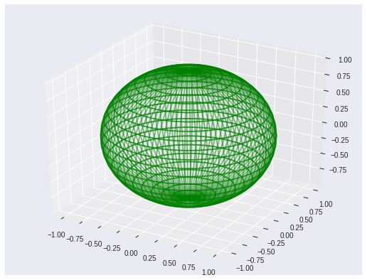
A (almost) parameterization of the sphere is
$$ \mathbf{x}(\phi, \theta) = (\sin \phi \cos \theta, \sin \phi \cos \phi, \cos \phi) $$
Note that there’s some bookkeeping to be done around the north and south pole: either nothing maps there (i.e., $\mathbf{x}: (0, 2\pi) \times (0, 2\pi) \rightarrow S$), meaning the sphere is not covered, or lots of points map there (i.e., $\mathbf{x}: [0, 2\pi] \times [0, 2\pi] \rightarrow S$), and $\mathbf{x}$ is not injective.
phi, theta = tf.meshgrid(tf.linspace(0., 2 * np.pi, 50), tf.linspace(0., 2. * np.pi, 50))
X = tf.sin(phi) * tf.cos(theta)
Y = tf.sin(phi) * tf.sin(theta)
Z = tf.cos(phi)
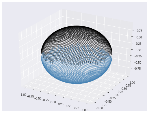
Two more parameterizations are
$$ \mathbf{x}_{\alpha}(x_1, x_2) = \sqrt{1 - x_1^2 - x_2^2} $$
$$ \mathbf{x}_{\beta}(x_1, x_2) = -\sqrt{1 - x_1^2 - x_2^2} $$
here there’s some care to be had around the equator.
x1, x2 = tf.meshgrid(tf.linspace(-1., 1., 100), tf.linspace(-1., 1., 100))
Xa = tf.sqrt(1 - x1 ** 2 - x2 ** 2)
Xb = -tf.sqrt(1 - x1 ** 2 - x2 ** 2)
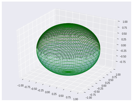
Since we assume our atlas is maximal, all three of these maps should actually be in it, as should all rotations of the maps, and subsets of the maps.
Calculus on manifolds
We conclude with calculus on manifolds. The rule of thumb here is to push everything through a parameterization or its inverse, and do your calculus in $R^n$.
Definition (differentiable map) Given two differentiable manifolds, $M_{\alpha}$ with atlas ${\mathbf{x}_{\alpha}}$ and $M_{\beta}$ with atlas ${\mathbf{y}_{\beta}}$, a map $f: M_{\alpha} \rightarrow M_{\beta}$ is differentiable at $p \in M_{\alpha}$ if there exists a parameterization $\mathbf{x} \in {\mathbf{x}_{\alpha}}$ and $\mathbf{y} \in {\mathbf{y}_{\beta}}$ so that $$ \mathbf{y}^{-1} \circ f \circ \mathbf{x} $$
is differentiable at $\mathbf{x}^{-1}(p)$.
Definition (differentiable curve) A differentiable function $\alpha: (-\epsilon, \epsilon) \subset \mathbb{R} \rightarrow M$ is called a differentiable curve in the manifold $M$.
Definition (tangent vector) Let $\alpha$ be a differentiable curve on $M$, $\alpha(0) = p \in M$, let $\mathcal{D}$ be the differentiable functions on $M$ at $p$, and let $f$ be an element of $\mathcal{D}$. The tangent vector to $\alpha$ is a function from $\mathcal{D} \rightarrow \mathbb{R}$, $$ \alpha’(0)f = \left. \frac{d(f \circ \alpha)}{dt} \right|_{t=0} $$ The set of all tangent vectors at $p$ is denoted $T_pM$.
Discussion The tangent vector to a curve at a point eats functions and returns a real number. We will give $T_pM$ the structure so that it is a vector space.
Example: This is the parabaloid from earlier, with a curve lifted onto it, and the point t=0 marked in red.
X, Y = tf.meshgrid(tf.linspace(-2., 2., 50), tf.linspace(-2., 2., 50))
hyperbolic_parabaloid = lambda x, y: 1 - x**2 + y**2 # look it up

t = tf.linspace(-1., 1., 100)
y = 1 + .5 * tf.cos(8 * t - 1)
f2 = hyperbolic_parabaloid(t, y)

with tf.GradientTape() as g:
    g.watch([X, Y])
    f = hyperbolic_parabaloid(X, Y)
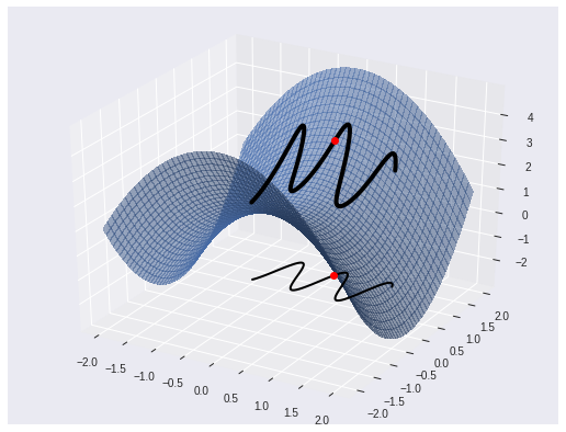
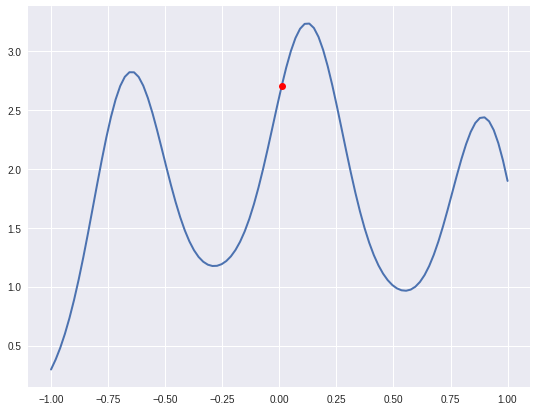
We can also look at the tangent vector to $\alpha$ of the height of the graph by plotting $f \circ \alpha : (-\epsilon, \epsilon) \rightarrow \mathbb{R}$:
The tangent vectors are a tangent space
If we write down a parameterization $\mathbf{x}: U \subset \mathbb{R}^n \rightarrow M$ of $M$ at $p = \mathbf{x}(0)$, then we can use the chain rule to write down the tangent vector to a curve $\alpha$ of a function $f$. Using the definition from earlier, $$ \alpha’(0)f = \left. \frac{d(f \circ \alpha)}{dt} \right|_{t=0}, $$
but $\alpha(t) = (x_1(t), \ldots, x_n(t))$, so
$$ \alpha’(0)f = \left. \frac{d}{dt} f(x_{1}(t), \ldots, x_{n}(t)) \right|_{t=0} $$
Applying the chain rule gives
$$ \alpha’(0)f = \sum_{j=1}^n x_i’(0) \left( \frac{\partial f}{\partial x_j} \right) = \left(\sum_{j=1}^n x_i’(0) \left( \frac{\partial}{\partial x_j} \right)_0 \right) f $$
It turns out (but can be checked!) that the vectors $\left( \frac{\partial}{\partial x_j} \right)_0$ are the tangent vectors of the coordinate curves in the parameterization given by $\mathbf{x}$. They define a basis of the vector space $T_pM$, associated with the parameterization $\mathbf{x}$.
One last theorem and definition
Definition (differential) Suppose you have a differentiable mapping $\varphi: M_1 \rightarrow M_2$ between manifolds, $p \in M_1$, then the differential of $\varphi$ at $p$, is denoted $d_p\varphi: T_pM_1 \rightarrow T_{\varphi(p)}M_2$, is defined as follows:
- Take a vector $\nu \in T_pM_1$
- Take a curve $\alpha : (-\epsilon, \epsilon) \rightarrow M_1$ with $\alpha(0) = p$ and $\alpha’(0) = \nu$
- Let $\beta = \varphi \circ \alpha$
- Define $d_p\varphi(\nu) = \beta’(0)$
It is a theorem to show that $d_p\varphi$ does not depend on the choice of $\alpha$.