See PyMC3 on GitHub here, the docs here, and the release notes here. This post is available as a notebook here.
I think there are a few great usability features in this new release that will help a lot with building, checking, and thinking about models. To give an introduction, I am going to to a bad job of implementing the “eight schools” model, and show how these new features help debug the model. I am using this particular model as one that is complicated enough to be interesting, but not too complicated.
1. Checking model initialization
This implementation has two different mistakes in it that we will find. First, the method Model.check_test_point is helpful to see if you have accidentally defined a model with 0 probability or with bad parameters:
J = 8
y = np.array([28.,  8., -3.,  7., -1.,  1., 18., 12.])
sigma = np.array([15., 10., 16., 11.,  9., 11., 10., 18.])

with pm.Model() as non_centered_eight:
    mu = pm.Normal('mu', mu=0, sd=5)
    tau = pm.HalfCauchy('tau', beta=5, shape=J)
    theta_tilde = pm.Normal('theta_t', mu=0, sd=1, shape=J)
    theta = pm.Deterministic('theta', mu + tau * theta_tilde)
    obs = pm.Normal('obs', mu=theta, sd=-sigma, observed=y)

non_centered_eight.check_test_point()
mu          -2.530000
tau_log__   -9.160000
theta_t     -7.350000
obs              -inf
Name: Log-probability of test_point, dtype: float64
Now that I see that obs has -inf log probability, I notice that I set the standard deviation to a negative number! quelle horreur! Let’s fix that and see if we can find other mistakes.
with pm.Model() as non_centered_eight:
    mu = pm.Normal('mu', mu=0, sd=5)
    tau = pm.HalfCauchy('tau', beta=5, shape=J)
    theta_tilde = pm.Normal('theta_t', mu=0, sd=1, shape=J)
    theta = pm.Deterministic('theta', mu + tau * theta_tilde)
    obs = pm.Normal('obs', mu=theta, sd=sigma, observed=y)

non_centered_eight.check_test_point()
mu           -2.53
tau_log__    -9.16
theta_t      -7.35
obs         -31.46
Name: Log-probability of test_point, dtype: float64
Everything looks ok now at the test point, at least!
2. Model Graphs
It takes an optional install (conda install -c conda-forge python-graphviz), but you can visualize your models in plate notation. This can be useful for sharing your model, or just checking that you implemented the right one.
pm.model_to_graphviz(non_centered_eight)
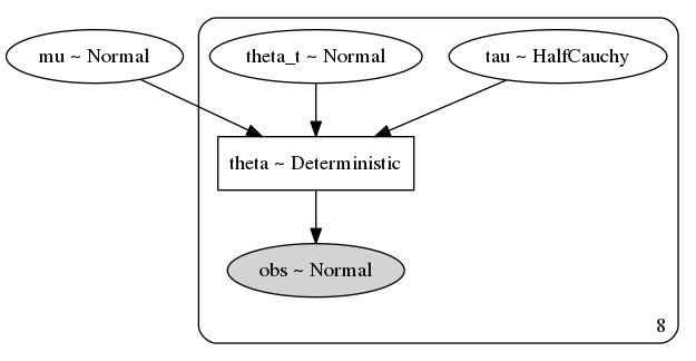
Oops! I meant for both mu and tau to be shared priors among the eight groups, but left an extra shape=J argument in there.
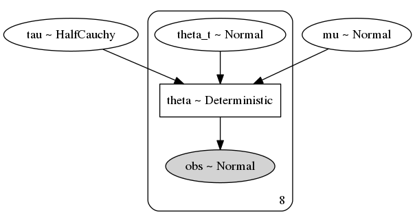
with pm.Model() as non_centered_eight:
    mu = pm.Normal('mu', mu=0, sd=5)
    tau = pm.HalfCauchy('tau', beta=5)
    theta_tilde = pm.Normal('theta_t', mu=0, sd=1, shape=J)
    theta = pm.Deterministic('theta', mu + tau * theta_tilde)
    obs = pm.Normal('obs', mu=theta, sd=sigma, observed=y)

pm.model_to_graphviz(non_centered_eight)
3. Sampling from the prior
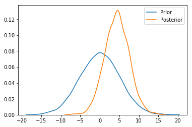
We can sample from the prior in the absence of data. This might seem like a small thing, but required a lot of refactoring along the way. Previously, this would be done by copy/pasting the model, deleting the observed arguments, and using MCMC. Now it can be done in the same model context, and is vectorized, running thousands of times faster. I am excited to see what tools and visualizations can be built around this, but in the meantime we can see how the presence of data effects our prior beliefs for the hierarchical mean here.
with non_centered_eight:
    prior = pm.sample_prior_predictive(5000)
    posterior = pm.sample()
Auto-assigning NUTS sampler...
Initializing NUTS using jitter+adapt_diag...
Multiprocess sampling (4 chains in 4 jobs)
NUTS: [theta_t, tau, mu]
Sampling 4 chains: 100%|██████████| 4000/4000 [00:02<00:00, 1897.82draws/s]
sns.distplot(prior['mu'], label='Prior', hist=False)
ax = sns.distplot(posterior['mu'], label='Posterior', hist=False)
ax.legend()
4. Nifty new progress bar
Check out also the progressbar above, which now shows you the total number of draws the sampler is doing, instead of just the first chain’s progress. The progressbar is actually the visible part of a change in multiprocessing. It removes (on OSX and Linux) the use of pickle to pass models around for multiprocessing, so you could use lambda in your models again if you really wanted.
5. Ordered transformation
There’s a new ordered transform which is handy for sampling from, for example, 1-d mixture models. I’ll quickly generate a mixture model and use some of the tricks above to fit it.
# Generate data
N_SAMPLES = 100
μ_true = np.array([-2, 0, 2])
σ_true = np.ones_like(μ_true)
z_true = np.random.randint(len(μ_true), size=N_SAMPLES)
y = np.random.normal(μ_true[z_true], σ_true[z_true])

with pm.Model() as mixture:
    μ = pm.Normal('μ', mu=0, sd=10, shape=3)
    z = pm.Categorical('z', p=np.ones(3)/3, shape=len(y))
    y_obs = pm.Normal('y_obs', mu=μ[z], sd=1., observed=y)
mixture.check_test_point()
μ         -9.66
z       -109.86
y_obs   -292.47
Name: Log-probability of test_point, dtype: float64
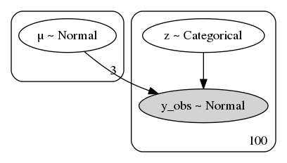
pm.model_to_graphviz(mixture)
with mixture:
    posterior = pm.sample()
Multiprocess sampling (4 chains in 4 jobs)
CompoundStep
>NUTS: [μ]
>CategoricalGibbsMetropolis: [z]
Sampling 4 chains: 100%|██████████| 4000/4000 [00:09<00:00, 405.95draws/s]
The acceptance probability does not match the target. It is 0.4428216460380929, but should be close to 0.8. Try to increase the number of tuning steps.
The gelman-rubin statistic is larger than 1.4 for some parameters. The sampler did not converge.
The estimated number of effective samples is smaller than 200 for some parameters.
pm.traceplot(posterior, varnames=['μ'], combined=True)
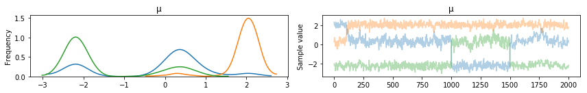
Notice the chains “jumping” between modes. This phenomena is called label switching. We can handle it with the ordered transform.
import pymc3.distributions.transforms as tr

with pm.Model() as mixture:
    μ = pm.Normal('μ', mu=0, sd=10, shape=3,
                  transform=tr.ordered,
                  testval=np.array([-1, 0, 1]))  # the `ordered` transform needs an initialization
                                                 # that is also ordered! PRs welcome!
    z = pm.Categorical('z', p=np.ones(3) / 3, shape=len(y))
    y_obs = pm.Normal('y_obs', mu=μ[z], sd=1., observed=y)
    posterior = pm.sample()
Multiprocess sampling (4 chains in 4 jobs)
CompoundStep
>NUTS: [μ]
>CategoricalGibbsMetropolis: [z]
Sampling 4 chains: 100%|██████████| 4000/4000 [00:15<00:00, 251.06draws/s]
The estimated number of effective samples is smaller than 200 for some parameters.
pm.traceplot(posterior, varnames=['μ'], combined=True)
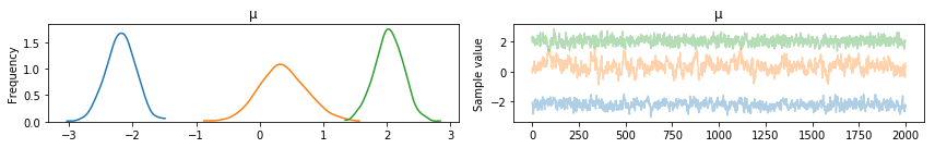
Look! No label switching! How cool!