Editors Note: These are a bit of an elaboration on some notes I took for the PyMC3 journal club on the very interesting new paper Generalizing Hamiltonian Monte Carlo with Neural Networks. These notes are pretty technical, and assume familiarity with Hamiltonian samplers (though there are reminders)! They aim to build intution, and perhaps serve as a fast first read before checking out the (very readable, and only 10 page) paper. As such, it sacrifices some details and correctness.
I have removed all the code from the post, but it is available as a Jupyter notebook here, if you are into that sort of thing.
One sentence summary: You can agument Hamiltonian Monte Carlo with six functions that might be able to handle different posteriors better, and we have a way to train a neural net to be those six functions.
The idea
Hamiltonian Monte Carlo had success in lifting a set of parameters $x\in \mathbb{R}^n$ to $\xi = (x, v) \in \mathbb{R}^{2n}$. The general idea of the algorithm was
Leapfrog ($\mathbf{L}$) and then flip ($\mathbf{F}$) the parameters: $$\xi \rightarrow \xi’=\mathbf{F}\mathbf{L}\xi$$ Caveat: I ignore the flip operator throughout this summary
Use the Metropolis acceptance criterion: $$A\left(\xi’|\xi\right) = \min \left(1, \frac{p(\xi’)}{p(\xi)}\left| \frac{\partial \mathbf{F}\mathbf{L} (\xi)}{\partial \xi} \right| \right)$$
The Jacobian of the leapfrog is 1 since it is volume preserving, and Hamiltonian dynamics should move along level sets in the probability space, so every proposal is accepted.
This paper proposes an extension of HMC, and feels like it actually has two main ideas:
- Extending the Leapfrog step If you do the book-keeping on the Jacobian, you can choose any six continuous functions (called $S$, $T$, $Q$, with subscript $v$ or $x$) and use them in the leapfrog step, while still having a valid MCMC algorithm.
- Optimizing the Leapfrog step The authors then propose using deep nets for these six functions, and fit them by optimizing the expected length of a step.
In context, this is interesting because one of the difficulties of Hamiltonian Monte Carlo is that it has lots of parameters, making tuning difficult. The NUTS sampler is wonderful in setting some of these paramters not only automatically, but reasonably optimally.
Extending the Leapfrog step
Recall that we assume $p(x) = e^{-U(x)}$. In this paper, rather than assuming a general kinetic energy function, $V(x, v)$, the authors set $V(x, v) = 0.5 |v|^2$. I use the general operator here so you can recognize it.
Now we wish to simulate Hamiltonian dynamics. That is,
$$
\begin{eqnarray}
\frac{d x}{dt} &=& \frac{\partial V}{\partial v}
\frac{d v}{dt} &=& -\frac{\partial U}{\partial x}
\end{eqnarray}
$$
We do this using a leapfrog integrator, which has a pleasant form. Fixing some step size $\epsilon$, we transform $(x, v)$ to $(x’, v’)$ by:
$$
\begin{eqnarray}
v^{\frac{1}{2}} &=& v - \frac{\epsilon}{2}\partial_xU(x)
x’ &=& x + \epsilon \partial_vV(x, v^{\frac{1}{2}})
v’ &=& v^{\frac{1}{2}} - \frac{\epsilon}{2}\partial_xU(x’)
\end{eqnarray}
$$
In addition to the pleasant properties of the Jacobian (it is 1) and conserving energy, note that in a loop, this turns into a half step for momentum, then full position and momentum steps, then a final half momentum step. I like that.
So this is the idea of this paper: instead of that first momentum update, we will use $$ v^{\frac{1}{2}} = v \odot e^{\frac{\epsilon}{2}S_v(\zeta)} - \frac{\epsilon}{2}\left(\partial_xU(x) \odot e^{\epsilon Q_v(\zeta)} + T_v(\zeta)\right) $$
The symbol $\odot$ is pointwise multiplication. If we wanted to be rigorous about linear algebra, $\odot$ is multiplication by a diagonal matrix, which is just scaling. $S_v$, $Q_v$, and $T_v$ are just continuous functions for now! Later they will be neural networks, but they do not have to be. $\zeta = (x, \partial_xU(x), t)$ is our state: it does not include $v$, but it does include $t$, and we could not figure out why.
In addition to using a similar trick on the position, we also update a subset of indices at a time. The paper does this in two steps, both looking like: $$ x’ = x \odot e^{\frac{\epsilon}{2}S_x(\zeta)} + \epsilon\left(\partial_vV(x, v) \odot e^{\epsilon Q_x(\zeta)} + T_x(\zeta)\right) $$ Note that you would do this twice on complementary indices, and in this case, $\zeta = (x, v, t)$. These steps could actually be done in parallel, but the indices are resampled each iteration.
This is followed by another “metaphorical half step”, as above.
It turns out (Appendix B) you can compute the Jacobian of this, and it only depends on $S_x$, $S_v$, and all the $\zeta$ state variables.
So now we have a leapfrog procedure that works for any choice of functions $S_v, Q_v, T_v, S_x, Q_x, T_x$, each of which accepts a bunch of state variables.
Optimizing the Leapfrog step
Now the authors model these six functions as neural nets, which depend on a set of parameters, $\theta$. In order to train these nets, we need to define a loss and a training method.
I am going to define two extra loss functions - the authors use just $\ell$ and $\mathcal{L}$. At a given point $\xi$, define the loss of jumping to $\xi’$ as
$$ l_{\lambda}(\xi, \xi’, A(\xi | \xi’)) = \frac{\lambda^2}{|\xi - \xi’|^2A(\xi | \xi’)}, $$
where $\lambda$ is a scale parameter.
Then the paper defines $$ \ell{\lambda} = l{\lambda} + \frac{1}{l_{\lambda}}. $$
Now, to make this loss depend on $\theta$ (remember that since those six functions are all neural nets, the parameters $\theta$ are really defining those six functions), and the probability distribution, we define the loss as an expectation over a probability distribution $p$:
$$ L_{p}(\theta) = \mathbb{E}_p \left[\ell_{\lambda}(\xi, \mathbf{F}\mathbf{L}_{\theta}\xi, A(\mathbf{F}\mathbf{L}_{\theta}\xi | \xi))\right]. $$
Now finally the objective function the authors define is a weighted average of this loss over the posterior and the initial distribution (which might be the prior). Intuitively, this is a weighted average of fast mixing and fast burn-in.
$$ \mathcal{L}(\theta) = L_p(\theta) + \lambda_b L_{q}(\theta), $$ where $p$ is the distribution we are drawing from, $q$ is the joint initial distribution (specifically, $q(\xi) = \pi_0(x) p_V(v | x) p(d)$, where $\pi_0$ is an initial distribution, $p_V$ is the momentum pdf, and $p(d)$ is a direction variable I am ignoring).
Training the neural nets
I quote from the paper, because this was hard to spot:
In Section 5.1, the Q, S, T are neural networks with 2 hidden layers with 10 (100 for the 50-d ICG) units and ReLU non-linearities. We train with Adam (Kingma & Ba, 2014) and a learning rate α = 10−3 . We train for 5,000 iterations with a batch size of 200.
I liked their training algorithm: the whole point of MCMC is to compute expectations, and so, very roughly, the algorithm is:
- Sample $N$ points $\xi_p$ from the initial distribution $q$ - these will be used for an expectation over $p$
Do the following $n$ times:
Sample $N$ points $\xi_q$ from the initial distribution - these wil be used for an expectation over $q$.
For each of the $N$ points, take a leapfrog step with both $\xi_p$ and $\xi_q$, and accumulate the loss $\mathcal{L}_{\theta}$. Actually accept or reject the proposal for $\xi_p$, so it mixes.
Adjust $\theta$ by the gradient of $\mathcal{L}$.
Profit.
Experiments
I recreated some of the experiments from the paper. This does not include their sampler (yet!) but does show when PyMC3’s samplers fail on these problems. Note that I am using a single chain for each experiment, which is not a great practice (but is at least illustrative). You would detect these in your own work by setting njobs=4, for example.
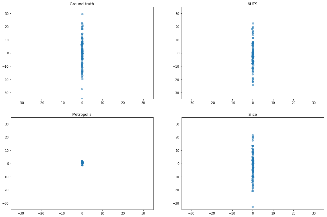
Ill-Conditioned Gaussian
Gaussian distribution with diagonal covariance spaced loglinearly between $10^{−2}$ and 10^2. This demonstrates that L2HMC can learn a diagonal inertia tensor.
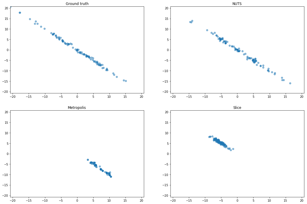
Strongly correlated Gaussian (SCG)
We rotate a diagonal Gaussian with variances $[10^2, 10^{−2}]$ by $\pi / 4$. This is an extreme version of
an example from Neal (2011). This problem shows that, although
our parametric sampler only applies element-wise transformations, it can adapt to structure which is
not axis-aligned.
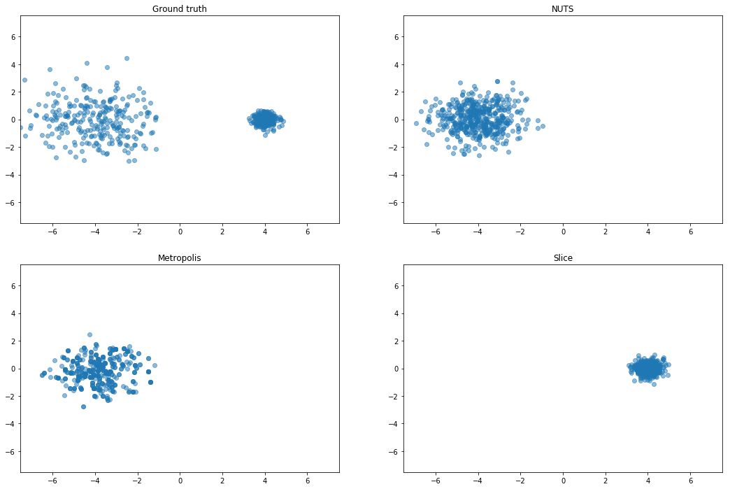
Mixture of Gaussians (MoG)
Mixture of two isotropic Gaussians with $\sigma^2 = 0.1$, and centroids
separated by distance 4. The means are thus about 12 standard deviations apart, making it almost
impossible for HMC to mix between modes.
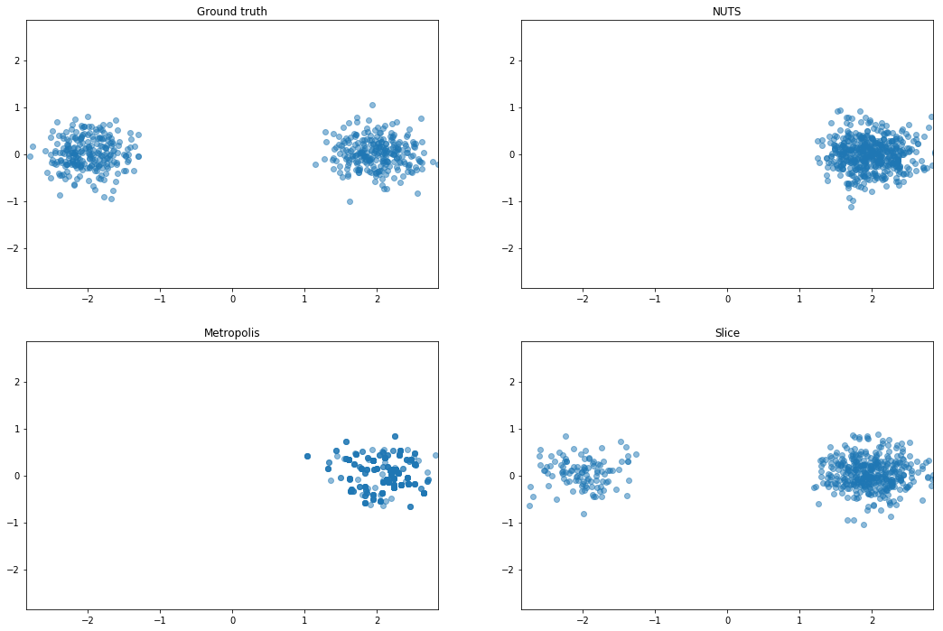
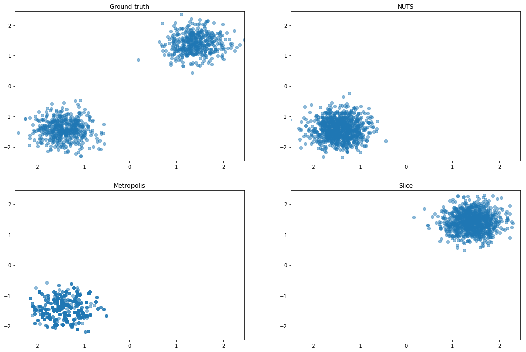
It looks like they also do an experiment with very two isotropic Gaussians and different scales. Might be something like this:
Curious about rotating the centers, since slice should not do well there
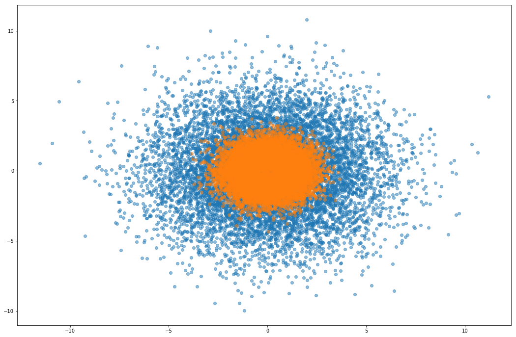
Rough Well
Similar to an example from Sohl-Dickstein et al. (2014), for a given $\eta > 0$, $U(x) = \frac{1}{2}x^Tx + \eta \sum_i \cos(\frac{x_i}{\eta})$. For small $\eta$ the energy itself is altered negligibly, but its gradient is perturbed by a high frequency noise oscillating between -1 and 1. In our experiments, we choose $\eta = 10^{−2}$.
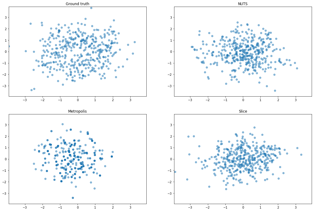
Confirm rough well is sampled reasonably
I don’t get anything out of the rough well experiments, so this is a sanity check that the rejection sampler is not just accepting everything or something. Orange is the rough well distribution, and blue are samples from the proposal distribution (a gaussian).